The Renormalisation Group: A Course for People Who Know a Little QFT

Physics looks different depending on how closely you look. Up close, water is molecules bumping into each other. From a metre away it is a smooth liquid with a density and a viscosity. Nobody needs the molecules to predict how it flows. The renormalisation group (RG for short) is the mathematics of that change of view. It tells you how the numbers in a theory must change when you step back and look from further away.

That one idea explains a surprising amount:

• why a magnet and a boiling liquid share exactly the same strange numbers near their critical points,

• why the electric charge of an electron looks bigger when you probe it harder,

• why quarks are almost free inside a proton but can never escape it,

• and why we can do physics at all without knowing what happens at the smallest scales.

First, one word: coarse-graining

The whole course keeps using one word, so here it is with a picture.

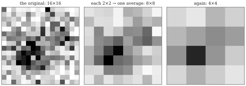
Coarse-graining a picture: replace every 2×2 square of pixels by one pixel with their average shade, then do it again. Fine detail is lost, but the big shapes survive.

For a magnet made of tiny arrows (spins) that point up or down, coarse-graining means taking a small block of neighbouring spins and replacing it with one big spin that points the way most of them point. It's a majority vote. The result is the same magnet, seen from further away.

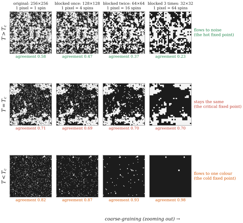
The whole course in one picture. A simulated magnet (the two colours are the two spin directions) is coarse-grained three times by majority vote, moving left to right. Too hot (top row) and the blocks drift towards noise: neighbours agree 0.58 of the time, then 0.47, 0.37, 0.23. Too cold (bottom row) and they drift to one colour: 0.82, 0.87, 0.93, 0.98. At exactly the critical temperature (middle row) the number barely moves: 0.71, 0.69, 0.70, 0.70. Something that doesn't change when you zoom out is called a fixed point and finding fixed points is what the RG does.

What you need to know first

You need calculus, a little complex analysis (what a pole is) and the idea that a field is a number at every point of space. It helps to have seen a path integral and a Feynman diagram once, but you don't need to be comfortable with them: Part 2 derives the Feynman rules from scratch, including where the propagator, the vertex, the minus signs and the symmetry factors come from. You don't need to have met a loop integral, a cutoff or the word "regularisation" before and you need no statistical mechanics beyond the Boltzmann factor \(e^{-E/k_BT}\).

The eight parts

How to use it

Read the parts in order, since each one builds on the last. Every part ends with exercises; try each one before you open its solution. Most take about ten minutes.

The interactive boxes run inside your own browser, so nothing is sent anywhere. They're kept light enough that your computer won't slow down and the magnet simulation pauses itself when you scroll away from it. When a widget sits next to a paragraph, playing with the widget is usually the quickest way to understand the paragraph.

If you only have one evening, read Parts 3 and 4. They contain the whole idea without any field theory.