
Renormalisation Group VI: The Wilson-Fisher Fixed Point
Part 6 of eight. previous: Wilson's shells · Course home · Glossary · next: Running couplings
In Part 5 the free field gave us the Gaussian fixed point and power counting showed that below four dimensions the quartic coupling pushes the system away from it. Now we switch \(u\) on and do Move 1, integrating out the shell, for real. It's a one-loop calculation and it's the heart of the work that earned Wilson the 1982 Nobel prize.
Integrating out the shell
Split the interaction using \(\phi=\phi_{\rm s}+\phi_{\rm f}\) and expand:
\[ \frac u{4!}\int\mathrm d^dx\,(\phi_{\rm s}+\phi_{\rm f})^4 = \frac u{4!}\int\mathrm d^dx\,\Big(\phi_{\rm s}^4 + 4\phi_{\rm s}^3\phi_{\rm f} + 6\phi_{\rm s}^2\phi_{\rm f}^2 + 4\phi_{\rm s}\phi_{\rm f}^3 + \phi_{\rm f}^4\Big). \]Two different integrals turn up from here on, so keep them apart. \(\int\mathrm d^dx\) runs over space, adding up the interaction at every point. \(\int_{\rm shell}\) runs over momentum, adding up the modes being removed, in the thin shell \(\Lambda/b<|\mathbf k|<\Lambda\). It is short for
\[ \int_{\rm shell}\;\equiv\;\int_{\Lambda/b<|\mathbf k|<\Lambda}\frac{\mathrm d^dk}{(2\pi)^d}, \]with the \((2\pi)^d\) there for the same reason as in Part 2: it is the price of a Fourier transform.
Treat \(u\) as small and average over the fast modes \(\phi_{\rm f}\), which behave like Gaussian random noise with the propagator \(G(k)=1/(k^2+r)\) in the shell. Here is where the formula below comes from. Write \(X=S_{\rm int}\), with the subscript on the bracket saying which fields are being averaged: \(\langle\cdot\rangle_{\rm f}\) means "average over the fast modes only, holding the slow ones fixed as though they were constants". Integrating out the fast modes then means
\[ e^{-S'[\phi_{\rm s}]} = e^{-S_0[\phi_{\rm s}]}\,\big\langle e^{-X}\big\rangle_{\rm f}. \]Every bracket from here to the end of the calculation is that same fast-mode average, so the subscript is dropped while the algebra is generic. Expand the exponential, \(\langle e^{-X}\rangle = 1-\langle X\rangle+\tfrac12\langle X^2\rangle-\dots\) then take the logarithm using \(\ln(1+y)=y-\tfrac12y^2+\dots\) with \(y=-\langle X\rangle+\tfrac12\langle X^2\rangle\). Keeping terms up to second order in \(X\):
\[ \ln\langle e^{-X}\rangle = -\langle X\rangle + \tfrac12\langle X^2\rangle - \tfrac12\langle X\rangle^2+\dots \]Since \(S' = S_0-\ln\langle e^{-X}\rangle\), this gives what's called the cumulant expansion:
\[ S'[\phi_{\rm s}] = S_0[\phi_{\rm s}] + \langle S_{\rm int}\rangle_{\rm f} - \tfrac12\Big(\langle S_{\rm int}^2\rangle_{\rm f} - \langle S_{\rm int}\rangle_{\rm f}^2\Big) + \dots \]Each term is a set of Feynman diagrams, with fast modes on the inside lines and slow fields on the outside ones.
The first-order term, piece by piece
Go through the five pieces of the expanded interaction one at a time (Tong §3.4 does the same). The fast modes are Gaussian noise, so we can average them with Part 5's rules: a pair of fast fields gives a propagator and an odd number gives zero.
\(\phi_{\rm s}^4\): no fast fields, so the average does nothing. This is just the old interaction for the slow modes, carried over unchanged.
\(4\phi_{\rm s}^3\phi_{\rm f}\): one fast field, so it averages to zero.
\(6\phi_{\rm s}^2\phi_{\rm f}^2\): two fast fields, averaging to \(\langle\phi_{\rm f}^2\rangle\). This is the only interesting piece at first order. It changes the mass, as we'll see next.
\(4\phi_{\rm s}\phi_{\rm f}^3\): three fast fields, so it averages to zero.
\(\phi_{\rm f}^4\): no slow fields at all. It gives a constant, which shifts the free energy but can't affect how the slow modes behave, so we drop it.
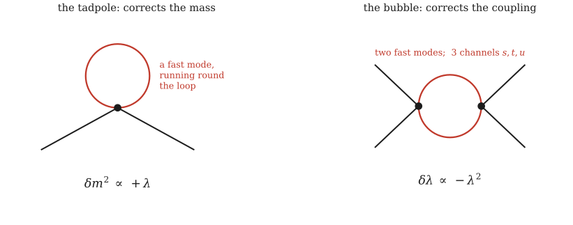
The two one-loop diagrams, with only fast (shell) modes going round the loop. The tadpole changes the mass. The bubble changes the coupling.
The mass. Take the \(6\phi_{\rm s}^2\phi_{\rm f}^2\) term from \(\langle S_{\rm int}\rangle_{\rm f}\) and average the two fast fields: \(\langle\phi_{\rm f}^2\rangle=\int_{\rm shell}G(k)\), a number. That leaves \(\frac{u}{4!}\cdot6\cdot\Big(\int_{\rm shell}G(k)\Big)\int\mathrm d^dx\,\phi_{\rm s}^2\). Comparing with the mass term \(\tfrac12\delta r\int\mathrm d^dx\,\phi_{\rm s}^2\):
\[ \delta r = \frac u2\int_{\rm shell}\frac{\mathrm d^dk}{(2\pi)^d}\,\frac1{k^2+r}. \]The shell is the only place the integral runs, because those are the only modes being removed. Its value is worked out below. Notice how the two integrals played different roles: the momentum one collapsed to a single number, which then multiplied the space integral that was already there. That is what makes it a shift of \(r\) rather than some new kind of term.
It helps to see the shell integral done for a finite step before taking the thin limit. In \(d=4\), with \(\mathrm d^4k/(2\pi)^4 = K_4\,k^3\,\mathrm d k\) and \(K_4=1/8\pi^2\), the same splitting as in Part 1 gives
\[ \delta r = \frac u2K_4\int_{\Lambda/b}^{\Lambda}\frac{k^3\,\mathrm d k}{k^2+r} = \frac{u}{32\pi^2}\left[\Big(1-\frac1{b^2}\Big)\Lambda^2 - r\ln\frac{\Lambda^2+r}{\Lambda^2/b^2+r}\right]. \]Now make the step thin, \(b=e^{\delta\ell}\) and keep terms to first order in \(\delta\ell\): \(1-b^{-2}\approx2\,\delta\ell\) and \(\ln\frac{\Lambda^2+r}{\Lambda^2e^{-2\delta\ell}+r}\approx\frac{2\Lambda^2\,\delta\ell}{\Lambda^2+r}\). So
\[ \delta r \approx \frac{u}{32\pi^2}\left[2\Lambda^2-\frac{2r\Lambda^2}{\Lambda^2+r}\right]\delta\ell = \frac{u}{16\pi^2}\,\frac{\Lambda^4}{\Lambda^2+r}\,\delta\ell = \frac u2K_4\,\frac{\Lambda^4}{\Lambda^2+r}\,\delta\ell, \]which is the thin-shell rule used below. (Both the finite-\(b\) formula and its thin limit were checked in Wolfram.)
The coupling. Take two vertices from \(-\tfrac12\langle S_{\rm int}^2\rangle_c\) (the subscript \(c\) means connected, explained a few lines below), keep two slow legs on each and join the rest with two fast propagators. Now count the ways. At each vertex, choose which 2 of the 4 legs are slow: that's \(\binom42^2=36\). Then join the two fast legs at vertex 1 to the two at vertex 2: that's 2 more ways. So there are \(72\) in all. The term is \(-\tfrac12\left(\frac u{4!}\right)^2\cdot72\Big(\int_{\rm shell}G(k)^2\Big)\int\mathrm d^dx\,\phi_{\rm s}^4 = -\frac{u^2}{16}\Big(\int_{\rm shell}G(k)^2\Big)\int\mathrm d^dx\,\phi_{\rm s}^4\), taken at zero outside momentum, which is fine for a plain \(\phi^4\) term. Matching to \(\frac{\delta u}{4!}\int\mathrm d^dx\,\phi_{\rm s}^4\):
\[ \delta u = -\frac{3u^2}{2}\int_{\rm shell}\frac{\mathrm d^dk}{(2\pi)^d}\,\frac1{(k^2+r)^2}. \]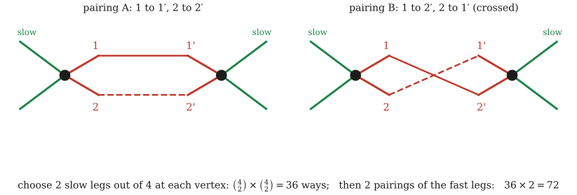
Where the 72 comes from. At each vertex, 2 of the 4 legs are slow (green) and 2 are fast (red). Wick's theorem joins the fast legs across in two ways, straight or crossed and both give the same bubble.
Why only the connected part, \(\langle S_{\rm int}^2\rangle-\langle S_{\rm int}\rangle^2\)? The pieces of \(\langle S_{\rm int}^2\rangle\) in which the two vertices don't share any fast line are exactly \(\langle S_{\rm int}\rangle^2\), so the subtraction removes them. That's lucky, because those pieces aren't local: they would describe two unrelated events far apart. What survives has the two vertices joined by fast lines, which is the bubble.
The minus sign matters: fluctuations weaken the coupling. In Part 7 this \(3/2\) turns out to be exactly what a completely different calculation needs, which is an independent check on the counting.
The shell integral. For a thin shell, \(b=e^{\delta\ell}\) with \(\delta\ell\) small, the integrand is the same all across the shell, so
\[ \int_{\Lambda/b}^{\Lambda}\frac{\mathrm d^dk}{(2\pi)^d}F(k) = K_d\,\Lambda^d\,F(\Lambda)\,\delta\ell,\qquad K_d=\frac{S_d}{(2\pi)^d}=\frac{2}{(4\pi)^{d/2}\Gamma(d/2)}. \]For reference: \(K_2=1/2\pi\), \(K_3=1/2\pi^2\) and \(K_4=1/8\pi^2\).
For a big step in four dimensions with \(r=0\), the bubble's shell integral is \(K_4\int_{\Lambda/b}^\Lambda\frac{k^3\mathrm d k}{k^4}=K_4\ln b\). So \(\delta u=-\frac{3u^2}{16\pi^2}\ln b\): each doubling of the length scale (\(b=2\)) takes off the same amount. This is the logarithm from Part 2, where every doubling of momentum added the same amount, now seen from the coarse-graining side.
The flow equations
Now do Moves 2 and 3 from Part 5, which multiply \(r\) by \(b^2\) and \(u\) by \(b^{4-d}\). (At one loop the field rescaling doesn't change, because no new \(k^2\phi^2\) term is created.) So after one thin step,
\[ r' = b^2\big(r+\delta r\big),\qquad u' = b^{4-d}\big(u+\delta u\big). \]With \(b=e^{\delta\ell}\) we have \(b^2\approx1+2\,\delta\ell\) and \(b^{4-d}\approx1+(4-d)\,\delta\ell\). Put in the shell results, \(\delta r=\frac u2K_d\Lambda^d\frac{1}{\Lambda^2+r}\,\delta\ell\) and \(\delta u=-\frac{3u^2}{2}K_d\Lambda^d\frac{1}{(\Lambda^2+r)^2}\,\delta\ell\) and keep only terms of first order in \(\delta\ell\):
\[ r'-r = \Big[2r + \frac{u}{2}\,\frac{K_d\Lambda^d}{\Lambda^2+r}\Big]\delta\ell,\qquad u'-u = \Big[(4-d)\,u - \frac{3u^2}{2}\,\frac{K_d\Lambda^d}{(\Lambda^2+r)^2}\Big]\delta\ell. \]Last, switch to the dimensionless couplings \(\tilde r=r/\Lambda^2\) and \(\tilde u=u\Lambda^{d-4}\), which is what "measure everything in units of the cutoff" means. (After Move 2 the cutoff is back at \(\Lambda\), so \(\Lambda\) is the same before and after the step.) Divide the first equation by \(\Lambda^2\) and multiply the second by \(\Lambda^{d-4}\). Then, for example, \(\frac{u}{\Lambda^2}\cdot\frac{\Lambda^d}{\Lambda^2+r}=\frac{u\Lambda^{d-4}}{1+r/\Lambda^2}=\frac{\tilde u}{1+\tilde r}\) and similarly for the other terms. Dividing by \(\delta\ell\) and letting it shrink to zero turns the differences into derivatives. Here \(\ell\) is "RG time", which increases as you zoom out towards long distances:
\[ \boxed{\;\frac{\mathrm d\tilde r}{\mathrm d\ell} = 2\tilde r + \frac{K_d}{2}\,\frac{\tilde u}{1+\tilde r},\qquad \frac{\mathrm d\tilde u}{\mathrm d\ell} = (4-d)\,\tilde u - \frac{3K_d}{2}\,\frac{\tilde u^2}{(1+\tilde r)^2}.\;} \]Read them term by term. The first term in each is the simple zoom-out scaling from Part 5. The second terms are the fluctuations we just integrated out: the coupling feeds the mass (the tadpole) and it weakens itself (the bubble).
These are the same equations as Melo's \(\beta_2,\beta_4\) once you flip the direction of RG time and the same as Tong's §3.4 in his notation.
What the flow says near the free point
Before finding the new fixed point, read off two things the equations already tell us.
Fluctuations lower the critical temperature. The critical line is where the mass doesn't run off, \(\mathrm d\tilde r/\mathrm d\ell=0\) at small \(\tilde u\). Setting \(2\tilde r+\frac{K_d}{2}\tilde u=0\) gives
\[ \tilde r_c = -\frac{K_d}{4}\,\tilde u+O(\tilde u^2). \]In mean-field theory the transition happens at \(r=0\). With fluctuations it needs \(r\) slightly negative, which means a slightly lower temperature. Fluctuations make ordering harder, so the magnet only orders once it's cooled a bit further than mean field predicts. (The exact solution of \(\mathrm d\tilde r/\mathrm d\ell=0\) is \(\tilde r_c=\tfrac12(\sqrt{1-K_d\tilde u}-1)\), which starts the same way; checked in Wolfram.)
In four dimensions the coupling dies slowly. With \(\epsilon=0\) and \(\tilde r\) small, \(\mathrm d\tilde u/\mathrm d\ell=-\frac{3\tilde u^2}{16\pi^2}\), whose solution is \(\tilde u(\ell)=\frac{\tilde u_0}{1+3\tilde u_0\ell/16\pi^2}\) (exercise 6.4). It goes to zero, but only like \(1/\ell\), which is \(1/\ln b\). That's the precise meaning of "marginally irrelevant".
The fixed points
Put \(\epsilon=4-d\) and look for places where both right-hand sides vanish. The new fixed point turns out to sit at \(\tilde u\) and \(\tilde r\) of size \(\epsilon\), so to leading order we can drop \(\tilde r\) in the denominators and use \(K_d\approx K_4=1/8\pi^2\):
Gaussian: \(\tilde r^*=\tilde u^*=0\).
Wilson-Fisher: \(\epsilon\tilde u^*=\frac{3K_4}{2}\tilde u^{*2}\), which gives
For \(\epsilon>0\) the new fixed point sits at a positive coupling, which is where a sensible \(\phi^4\) theory lives. As \(\epsilon\to0\) it merges into the Gaussian one.
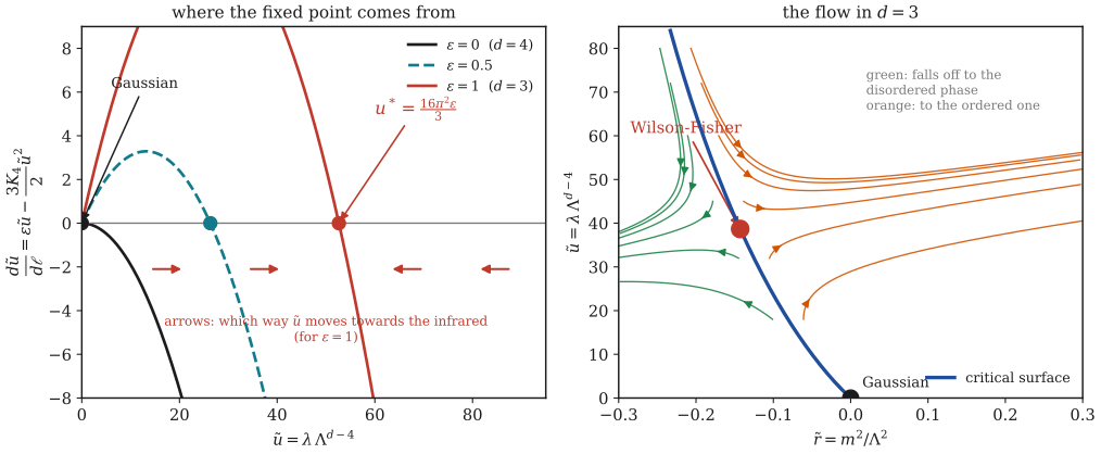
Left: the right-hand side of the \(\tilde u\) equation. In \(d=4\) (black) it's negative for every \(\tilde u>0\), so the coupling always shrinks and the only fixed point is \(\tilde u=0\). For \(\epsilon>0\) the curve crosses zero a second time, at the Wilson-Fisher point. Right: paths of the full one-loop equations in \(d=3\), worked out numerically. The critical surface (blue) runs from the Gaussian point into Wilson-Fisher. The red dot sits at \(\tilde u\approx38.7\), not \(52.6\), because these equations solved exactly (rather than only to first order in \(\epsilon\)) put the fixed point in a slightly different place. The two agree as \(\epsilon\to0\) and differ at order \(\epsilon^2\), where one loop isn't accurate anyway.
Exponents
Linearise around Wilson-Fisher. Write \(\tilde r=\tilde r^*+\delta r\) and \(\tilde u=\tilde u^*+\delta u\) and expand both flow equations to first order in \(\delta r\) and \(\delta u\). The four partial derivatives, evaluated at the fixed point and kept to first order in \(\epsilon\), are:
\(\dfrac{\partial\dot r}{\partial r}=2-\dfrac{K_4\tilde u^*}{2(1+\tilde r^*)^2}\approx2-\dfrac{K_4}{2}\cdot\dfrac{2\epsilon}{3K_4}=2-\dfrac\epsilon3\),
\(\dfrac{\partial\dot r}{\partial u}=\dfrac{K_4}{2(1+\tilde r^*)}\approx\dfrac{K_4}{2}\Big(1+\dfrac\epsilon6\Big)\),
\(\dfrac{\partial\dot u}{\partial r}=\dfrac{3K_4\tilde u^{*2}}{(1+\tilde r^*)^3}\), which is of order \(\epsilon^2\), so drop it,
\(\dfrac{\partial\dot u}{\partial u}=\epsilon-\dfrac{3K_4\tilde u^*}{(1+\tilde r^*)^2}\approx\epsilon-2\epsilon=-\epsilon\).
So
\[ \frac{\mathrm d}{\mathrm d\ell}\begin{pmatrix}\delta r\\ \delta u\end{pmatrix} = \begin{pmatrix}2-\frac\epsilon3 & \frac{K_4}{2}\big(1+\frac\epsilon6\big)\\ 0 & -\epsilon\end{pmatrix}\begin{pmatrix}\delta r\\ \delta u\end{pmatrix}. \]This is the same matrix as Tong's §3.5.1 (in his units) and Melo's (with RG time reversed). It's triangular, so its eigenvalues are just the diagonal entries. Its eigenvectors tell you which combinations of \(\delta r\) and \(\delta u\) grow or shrink:
The relevant eigenvector is \((1,0)\): a pure change of \(r\), which is a change of temperature.
The irrelevant eigenvector is about \(\big(-\tfrac{K_4}{4},1\big)\): move \(u\) by one unit and \(r\) by \(-K_4/4\). That's exactly the slope of the critical line \(\tilde r_c=-\frac{K_4}4\tilde u\) we found near the free point. So the irrelevant direction points along the critical surface, as it must: moving along the critical surface doesn't take you off criticality.
(The matrix, eigenvalues and eigenvectors were all checked in Wolfram.) The eigenvalues are
\[ y_t = 2-\frac\epsilon3, \qquad y_u=-\epsilon. \]That's one relevant direction (temperature) and one irrelevant one, exactly what a critical point should have. The Gaussian point has lost: there both rates are positive (\(2\) and \(+\epsilon\)), so you can't reach it by tuning just one knob. Every critical Ising system in \(d<4\) flows to Wilson-Fisher. The exponents follow:
\[ \nu = \frac1{y_t} = \frac12+\frac\epsilon{12}+O(\epsilon^2),\qquad \gamma = \nu(2-\eta) = 1+\frac\epsilon6+O(\epsilon^2), \]because \(\eta\) only appears at two loops, \(\eta=\epsilon^2/54\).
Why η is zero at one loop
The exponent \(\eta\) measures how the field's own scaling is changed by interactions. At one loop, the only correction to the two-point function is the tadpole and the tadpole doesn't depend on the outside momentum \(p\) at all: its loop never touches \(p\). So it can only shift the mass \(r\), never the \(p^2\) stiffness term. The field rescaling of Move 3 stays exactly as for the free field and \(\eta=0\). The first diagram that does depend on \(p\) is the two-loop "sunset", with three lines between two vertices and that's where \(\eta=\epsilon^2/54\) comes from.
All the exponents
With \(\eta=0\), the field's scaling is the free one, so the magnetic field's exponent is still \(y_h=\frac{d+2}{2}=3-\frac\epsilon2\). Together with \(y_t=2-\frac\epsilon3\), the formulas from Part 4 give every exponent. Expanding each to first order in \(\epsilon\):
\[ \begin{aligned} \nu&=\frac{1}{y_t}=\frac12+\frac{\epsilon}{12}, & \alpha&=2-\frac{d}{y_t}=\frac{\epsilon}{6}, & \beta&=\frac{d-y_h}{y_t}=\frac12-\frac{\epsilon}{6},\\ \gamma&=\frac{2y_h-d}{y_t}=1+\frac{\epsilon}{6}, & \delta&=\frac{y_h}{d-y_h}=3+\epsilon, & \eta&=0. \end{aligned} \]For example, \(\beta=\frac{(4-\epsilon)-(3-\epsilon/2)}{2-\epsilon/3}=\frac{1-\epsilon/2}{2(1-\epsilon/6)}\approx\frac12\big(1-\frac\epsilon2\big)\big(1+\frac\epsilon6\big)\approx\frac12-\frac\epsilon6\). (All six were expanded in Wolfram.)
Everything above was checked in Wolfram:
betam = 2 m2 + Kd4 u/(2 (1 + m2));
betau = eps u - 3 Kd4 u^2/(2 (1 + m2)^2);
us  = u /. Last[Solve[eps u - 3 Kd4 u^2/2 == 0, u]];        (* 2 eps/(3 Kd4) *)
m2s = m2 /. First[Solve[2 m2 + Kd4 us/2 == 0, m2]];        (* -eps/6 *)
yt  = Simplify[D[betam, m2] /. {m2 -> 0, u -> us}]          (* 2 - eps/3 *)
Series[1/yt, {eps, 0, 1}]                                   (* 1/2 + eps/12 *)
Simplify[D[betau, u] /. {m2 -> 0, u -> us}]                 (* -eps *)
Simplify[2/((4 Pi)^(4/2) Gamma[4/2]) - 1/(8 Pi^2)]          (* 0: K_4 = 1/(8 Pi^2) *)
How good is it?
Set \(\epsilon=1\) for three dimensions. One is not a small number and the expansion has no right to work there. Wilson and Fisher gave their 1972 paper the joking title "Critical exponents in 3.99 dimensions", as if \(\epsilon=0.01\). And yet:
| \(\nu\) | \(\alpha\) | \(\beta\) | \(\gamma\) | \(\delta\) | \(\eta\) | |
|---|---|---|---|---|---|---|
| mean field (Gaussian) | 0.5 | 0 | 0.5 | 1 | 3 | 0 |
| one loop, \(\epsilon=1\) | 0.583 | 0.167 | 0.333 | 1.167 | 4 | 0 |
| 3D Ising (conformal bootstrap) | 0.6300 | 0.1101 | 0.3265 | 1.2371 | 4.7898 | 0.0363 |
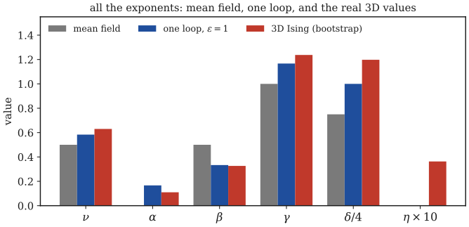
Every exponent moves from its mean-field value towards the true 3D value. The one-loop \(\beta=1/3\) is remarkably close to the real \(0.3265\). (\(\delta\) is divided by 4 and \(\eta\) multiplied by 10 so they fit on the same scale.)
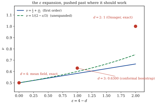
The one-loop \(\nu\) against \(\epsilon\). It moves away from mean field in the right direction and gets most of the way to the true 3D value. At \(\epsilon=2\) (the 2D Ising model) it's far off, as you'd expect. Adding more loops brings the 3D numbers within a fraction of a percent.
The first correction takes \(\nu\) two-thirds of the way from mean field to the true value. The deeper result doesn't depend on the numbers at all: below four dimensions the exponents are not mean-field and they are universal, fixed by just the dimension and the symmetry.
There is a second road to the same fixed point, one that never writes \(\epsilon\) down at all. It is worth walking, because it reaches three dimensions directly.
Three dimensions without an ε expansion
The \(\epsilon\) expansion earns its answers by staying near four dimensions, where the fixed point sits at small coupling. Three dimensions can also be attacked head on, by giving up the expansion in exchange for a different approximation: keep the dimension exact at \(d=3\) and approximate the shape of the theory instead.
Keep the whole potential, not two numbers
Look at what we actually tracked in this part: \(r\) and \(u\). That is the same as saying the potential
\[ U(\phi)=\tfrac12 r\phi^2+\frac{u}{4!}\phi^4 \]is described by two numbers. The RG step made \(\phi^6\), \(\phi^8\) and everything above as well. We dropped them, because power counting said they are irrelevant near four dimensions. In three dimensions that is an assumption, not a theorem.
So do not drop them. Follow the whole function \(U(\phi)\) as the scale changes. This was Wilson's own picture. Its modern form is an exact equation written down by Wetterich in 1993.
The exact equation
\[ \boxed{\;\partial_t\Gamma_k=\frac12\,\mathrm{Tr}\left[\big(\Gamma^{(2)}_k+R_k\big)^{-1}\partial_tR_k\right],\qquad t=\ln k.\;} \]One line, six symbols. Here is each of them.
The equation looks like a one-loop formula, because it is one loop, but taken with the full propagator instead of the free one. That is the whole trick, so it is exact. Nothing was expanded in a small coupling. Nothing was expanded in \(\epsilon\).
The local potential approximation
An exact equation for a whole function of two variables is not something you solve on paper. You truncate it. The simplest useful truncation keeps the kinetic term fixed at its classical form, letting only the potential flow:
\[ \Gamma_k=\int\mathrm d^dx\left[\tfrac12(\partial\phi)^2+U_k(\phi)\right]. \]That is the local potential approximation, or LPA. Take Litim's regulator, \(R_k(q)=(k^2-q^2)\theta(k^2-q^2)\), which fills the momentum integral in exactly. Write the potential in the dimensionless variable \(\rho=\phi^2/2\). Then the whole thing collapses to one equation:
\[ \partial_t u=-d\,u+(d-2)\,\rho\,u'+\frac{c_d}{1+u'+2\rho u''},\qquad c_d=\frac{K_d}{d},\quad K_d=\frac{2}{(4\pi)^{d/2}\Gamma(d/2)}. \]Read it left to right:
\(-d\,u\) is plain dimensional analysis. The potential has mass dimension \(d\), so measuring it in units of \(k\) costs this term.
\((d-2)\rho u'\) is the same thing for the field, since \([\phi]=(d-2)/2\) and \(\rho=\phi^2/2\).
the last term is the only place where any physics happens. It is the loop. The denominator is the inverse propagator at scale \(k\) with the real curvature of the potential in it. In the free theory \(u'=u''=0\) and the term is a constant.
Now put \(d=3\) in and never mention \(\epsilon\) again.
Solving it
Expand the potential around its own minimum \(\kappa\), which moves as the flow goes on:
\[ u(\rho)=\sum_{n=2}^{M}\frac{\lambda_n}{n!}\,(\rho-\kappa)^n,\qquad u'(\kappa)=0. \]Keeping \(M\) couplings means keeping the potential up to \(\phi^{2M}\). \(M=2\) is exactly this part's truncation: a mass plus a quartic. \(M=3\) adds \(\phi^6\), \(M=4\) adds \(\phi^8\) and so on. Set every flow to zero, which gives the fixed point, then linearise around it and read the exponents off the eigenvalues, exactly as in the "Exponents" section above.
Here is the whole solver. It is short enough to read in one sitting, because the only real work is Taylor arithmetic in \(x=\rho-\kappa\).
from math import factorial, pi
import numpy as np
from scipy.optimize import fsolve
from scipy.special import gamma as Gamma

Kd = lambda d: 2.0 / ((4 * pi) ** (d / 2) * Gamma(d / 2))

def rhs(y, d, M):                      # Taylor coefficients of the flow
    kap, lams = y[0], y[1:]            # u = sum_n lam_n x^n / n!
    c = Kd(d) / d
    u, up, upp = (np.zeros(M + 1) for _ in range(3))
    for i, n in enumerate(range(2, M + 1)):
        u[n]      += lams[i] / factorial(n)
        up[n - 1] += lams[i] / factorial(n - 1)
        upp[n - 2]+= lams[i] / factorial(n - 2)
    def times_rho(f):                  # rho = kappa + x
        out = kap * f.copy(); out[1:] += f[:-1]; return out
    D = np.zeros(M + 1); D[0] = 1.0
    D += up + 2 * times_rho(upp)
    E = np.zeros(M + 1); E[0] = 1 / D[0]        # 1/D as a series
    for k in range(1, M + 1):
        E[k] = -sum(D[j] * E[k - j] for j in range(1, k + 1)) / D[0]
    return -d * u + (d - 2) * times_rho(up) + c * E

def flow(y, d, M):
    R, lams = rhs(y, d, M), y[1:]
    dkap = -R[1] / lams[0]             # hold the minimum at the minimum
    dl = [R[n] * factorial(n) + (lams[i + 1] * dkap if i + 1 < len(lams) else 0)
          for i, n in enumerate(range(2, M + 1))]
    return np.concatenate(([dkap], dl))

y = np.array([0.03, 7.5])              # then fsolve(flow, y); the
                                       # exponents are -eig(Jacobian)
Run at 40 digits with mpmath, in \(d=3\), it gives:
| couplings kept \(M\) | potential up to | \(\nu\) | \(\omega\) |
|---|---|---|---|
| 2 | \(\phi^4\) | 0.500000 | 0.333333 |
| 3 | \(\phi^6\) | 0.728992 | 1.074990 |
| 4 | \(\phi^8\) | 0.650574 | 0.598864 |
| 5 | \(\phi^{10}\) | 0.644691 | 0.644426 |
| 6 | \(\phi^{12}\) | 0.649847 | 0.661194 |
| 8 | \(\phi^{16}\) | 0.649481 | 0.655182 |
| 10 | \(\phi^{20}\) | 0.649576 | 0.655796 |
| 13 | \(\phi^{26}\) | 0.649561 | 0.655754 |
| published LPA value | whole function | 0.649562 | 0.655746 |
| true 3D Ising | 0.6300 | 0.8303 |
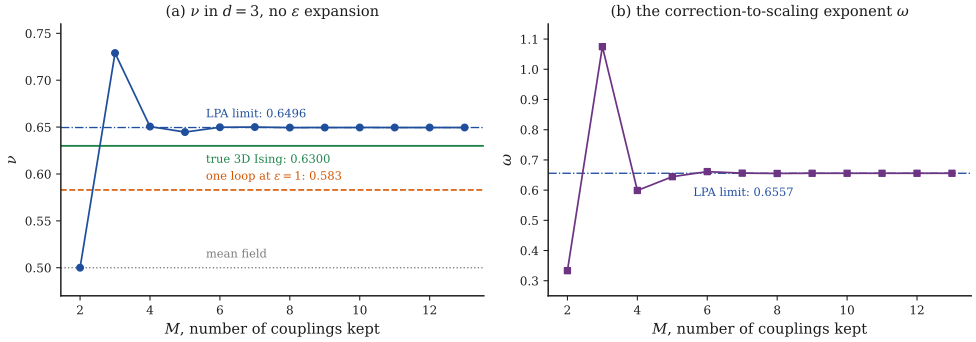
(a) Keeping two couplings in three dimensions gives exactly mean field. Keeping three overshoots badly. From four onwards the answer settles on \(0.6496\), which is past the one-loop \(\epsilon=1\) value and closer to the truth, though it overshoots it. (b) The same for \(\omega\).
Two couplings in three dimensions give exactly mean field. Not approximately: the \(M=2\) fixed point can be solved in closed form (Exercise 6.5) and its eigenvalues are exactly \(2\) and \(-\tfrac13\), so \(\nu=\tfrac12\) and \(\omega=\tfrac13\). The interesting physics in the last table came from the way the \(\epsilon\) expansion orders the terms, rather than from the two couplings themselves, which on their own carry no information about three dimensions.
The sequence converges, to a number that can be looked up. Litim computed the LPA exponents with this regulator in 2002 and found \(\nu=0.649562\) with \(\omega=0.655746\). The table lands on \(0.649561\) and \(0.655754\): six digits of agreement on \(\nu\), which is what makes a number like this worth quoting.
It is better than one loop. It is still not right. The whole ladder of methods for \(\nu\) in three dimensions:
| method | \(\nu\) | error |
|---|---|---|
| mean field | 0.5 | \(-20.6\%\) |
| one loop at \(\epsilon=1\) | 0.583 | \(-7.5\%\) |
| LPA in \(d=3\) | 0.6496 | \(+3.1\%\) |
| derivative expansion, order \(\partial^2\) | 0.6278 | \(-0.35\%\) |
| derivative expansion, order \(\partial^4\) | 0.63057 | \(+0.09\%\) |
| derivative expansion, order \(\partial^6\) | 0.63007 | \(+0.02\%\) |
| conformal bootstrap | 0.629971(4) |
What the LPA is still missing
The leftover 3% is not the truncation. \(M=13\) is converged to six digits. It is the local potential approximation itself.
The giveaway is \(\eta\). The LPA froze the kinetic term at \(\tfrac12(\partial\phi)^2\), so the field never picks up any extra scaling, so \(\eta=0\) exactly. The true value is \(0.0363\). The same crudeness shows up in \(\omega\), which comes out at \(0.66\) against the true \(0.83\): a 21% miss, much worse than \(\nu\)'s 3%. Both improve together once the kinetic term is allowed to flow.
The cure is to stop freezing the kinetic term. Let a factor \(Z_k\) in front of \((\partial\phi)^2\) flow too, which is called LPA\('\) and gives a nonzero \(\eta\). Keeping more derivative terms in a controlled sequence is the derivative expansion, whose numbers are in the table above: by order \(\partial^6\) it agrees with the conformal bootstrap to five digits. The small parameter there is not \(\epsilon\), it is roughly \(1/4\) to \(1/9\), which is why it behaves so much better at \(\epsilon=1\).
Three checks on the numbers
A calculation this short is easy to get quietly wrong, so it is worth pinning down from three directions.
Against the \(\epsilon\) expansion. Run near four dimensions, where the expansion of the last section is trustworthy, the same equation must reproduce \(\nu=\tfrac12+\tfrac\epsilon{12}\). It does, with the gap shrinking like \(\epsilon^2\): \(0.0005\) at \(\epsilon=0.1\), \(0.0021\) at \(\epsilon=0.2\), \(0.0135\) at \(\epsilon=0.5\). The middle pair differ by a factor \(6.4\) where \(\epsilon^2\) predicts \(6.25\).
Against pen and paper. The \(M=2\) fixed point is solvable by hand (Exercise 6.5), at \(\kappa^*=4c_3/3\) and \(\lambda_2^*=3/16c_3\). Those come to \(0.0225158\) and \(11.1033\), which is what the table above reports to every digit it prints.
Against the literature. Litim's published LPA values for this regulator, quoted above.
Magnets with more components: the O(N) models
Real magnets don't all have up/down spins. In some, each spin is an arrow free to point anywhere in a plane (\(N=2\), like superfluid helium), or anywhere in space (\(N=3\), the Heisenberg magnet). The field becomes a vector \(\boldsymbol\phi=(\phi_1,\dots,\phi_N)\) and the interaction is \(\frac{u}{4!}(\boldsymbol\phi\cdot\boldsymbol\phi)^2\). The whole calculation goes through with only the counting changed, so it's worth doing that counting properly.
Write the interaction as \(\frac u{4!}\,V_{abcd}\,\phi_a\phi_b\phi_c\phi_d\) (repeated indices summed), where the symmetric tensor
\[ V_{abcd}=\tfrac13\big(\delta_{ab}\delta_{cd}+\delta_{ac}\delta_{bd}+\delta_{ad}\delta_{bc}\big) \]reproduces \((\boldsymbol\phi\cdot\boldsymbol\phi)^2\). A fast propagator now carries a \(\delta_{ab}\): a fast \(\phi_a\) can only pair with a fast \(\phi_a\).
The tadpole. Two legs of one vertex are joined, so we need \(V_{abmm}\) (summed over \(m\)). Each term of \(V\) gives: \(\delta_{ab}\delta_{mm}=N\delta_{ab}\), \(\delta_{am}\delta_{bm}=\delta_{ab}\) and \(\delta_{am}\delta_{bm}=\delta_{ab}\). So \(V_{abmm}=\frac{N+2}3\,\delta_{ab}\), which for \(N=1\) is 1. So the tadpole is multiplied by \(\frac{N+2}{3}\):
\[ \delta r=\frac{N+2}{3}\cdot\frac u2\int_{\rm shell}G(k)=\frac{N+2}{6}\,u\int_{\rm shell}G. \]The bubble. Two slow legs at each vertex and two fast lines between them, so we need \(T_{ijkl}=V_{ijmn}V_{klmn}\). Multiply out the \(3\times3=9\) products of deltas. One product gives \(\delta_{mm}=N\) times \(\delta_{ij}\delta_{kl}\), four more also give \(\delta_{ij}\delta_{kl}\) and the last four give \(\delta_{ik}\delta_{jl}\) or \(\delta_{il}\delta_{jk}\) twice each:
\[ T_{ijkl}=\tfrac19\Big[(N+4)\,\delta_{ij}\delta_{kl}+2\,\delta_{ik}\delta_{jl}+2\,\delta_{il}\delta_{jk}\Big]. \]Since all four slow fields sit at the same point, only the part of \(T\) that's symmetric in all four indices matters. Symmetrising makes each of the three delta-pairs equally weighted, which gives \(\frac{(N+4)+2+2}{3}\) of each, so \(T\to\frac{N+8}{9}V\). The bubble is multiplied by \(\frac{N+8}9\):
\[ \delta u=-\frac{N+8}{9}\cdot\frac{3u^2}{2}\int_{\rm shell}G(k)^2=-\frac{N+8}{6}\,u^2\int_{\rm shell}G^2. \](I also checked both factors by brute-force tensor contraction on a computer for \(N=1\) to \(5\).) Tong has a nice way to see the \(N\) in these factors: a closed loop of fast modes can carry any of the \(N\) components, so every closed loop brings a factor of \(N\).
The flow equations become
\[ \frac{\mathrm d\tilde r}{\mathrm d\ell}=2\tilde r+\frac{N+2}{6}K_d\frac{\tilde u}{1+\tilde r},\qquad \frac{\mathrm d\tilde u}{\mathrm d\ell}=\epsilon\tilde u-\frac{N+8}6K_d\frac{\tilde u^2}{(1+\tilde r)^2}, \]with the fixed point at \(\tilde u^*=\frac{6\epsilon}{(N+8)K_4}\) and
\[ y_t=2-\frac{N+2}{N+8}\,\epsilon,\qquad \nu=\frac12+\frac{N+2}{4(N+8)}\,\epsilon. \]These match Tong §4.2. Different \(N\) gives a different fixed point and so a different universality class. The symmetry of the order parameter is one of the few things a fixed point remembers about the microscopic world.
Play with the flow
The widget integrates the full one-loop equations above. Click anywhere to start a theory at that point and watch where it flows. Drag \(\epsilon\) and watch the Wilson-Fisher point split off from the Gaussian one at \(\epsilon=0\). The readout gives the first-order \(\epsilon\) results in bold (these are the trustworthy ones) and, underneath, the exact zero of the truncated equations, which differs at order \(\epsilon^2\).
Things to try. Set \(\epsilon=0\) and click near the vertical axis: the paths creep down towards zero coupling, very slowly (the marginal case). Set \(\epsilon=1\) and click just left and just right of the blue line: the two paths travel side by side towards Wilson-Fisher, then split into opposite phases. The time they spend near the fixed point is the critical region.
Exercises
Show solution
Show solution
Show solution
Show solution
Show solution
The minimum stays at the minimum only if \(\dot\kappa=-R'(\kappa)/\lambda=0\), which gives \(\kappa=3c/D^2\) in \(d=3\). Setting \(\dot\lambda=R''(\kappa)=0\) gives \(1=18c\lambda/D^3\). Write \(z=2\kappa\lambda\), so \(D=1+z\). Substituting, \(z=2\cdot\frac{3c}{(1+z)^2}\cdot\frac{(1+z)^3}{18c}=\frac{1+z}{3}\), hence \(z=\tfrac12\) and \(D=\tfrac32\). Then
\[ \kappa^*=\frac{4c}{3},\qquad \lambda^*=\frac{3}{16c},\qquad c=\frac{K_3}{3}=0.0168866\dots \]so \(\kappa^*=0.0225158\) and \(\lambda^*=11.1033\). For the eigenvalues, use \(\dot\kappa=-\kappa+3c/D^2\) and \(\dot\lambda=-\lambda+18c\lambda^2/D^3\) with \(D=1+2\kappa\lambda\). The four partial derivatives at the fixed point give a matrix with trace \(-\tfrac53\) and determinant \(-\tfrac23\), whose eigenvalues are \(-2\) and \(+\tfrac13\). Flipping the sign for the convention \(\theta=-\,\)(eigenvalue) gives \(\theta=2\), so \(\nu=1/2\), with the irrelevant one at \(\omega=\tfrac13\).
Worth noticing: for general \(d\) the same algebra gives \(\lambda^*\propto(4-d)\), so this fixed point merges with the Gaussian one exactly at four dimensions. It is the Wilson-Fisher fixed point, seen from a different direction.
Show solution
Now read them off. \(n=1\) is the mass term \(\phi^2\), giving \(\theta_1=2\): relevant in any dimension, which is the fine tuning of the temperature. \(n=2\) is \(\phi^4\), giving \(\theta_2=4-d=\epsilon\): marginal at four dimensions, relevant just below, which is precisely why the Wilson-Fisher fixed point splits off there. \(n=3\) is \(\phi^6\), giving \(\theta_3=6-2d=2\epsilon-2\), irrelevant for small \(\epsilon\), which is the licence this part used to drop it. Part 5's power counting has come back out of a functional equation, with nothing put in by hand.