
Renormalisation Group VIII: Effective Field Theory
Part 8 of eight. previous: Running couplings · Course home · Glossary
We now have the machinery. This last part is about what it means. In short: the RG explains why we can do physics at all without knowing the final theory and it tells us which questions about very short distances the everyday world can and can't answer.
Why physics works: decoupling
Go back to the power counting of Part 5. A coupling \(g\) with negative mass dimension, \([g]=-p<0\), is irrelevant. Its effect at energy \(E\) is suppressed by \((E/\Lambda)^p\), where \(\Lambda\) is the scale where it came from. Run the flow down from very high energy and every irrelevant coupling fades away. What's left at low energy is a short list, the relevant and marginal couplings, no matter what the high-energy theory was.
That's why chemistry doesn't need quarks and why the Navier-Stokes equation has two parameters instead of \(10^{23}\). It's also why heavy particles decouple: a particle of mass \(M\) affects physics at \(E\ll M\) only by shifting the low-energy couplings, plus corrections suppressed by powers of \(E/M\). This is the Appelquist-Carazzone theorem. The ladder of theories in Part 1 is the RG flow drawn as a picture.
The best example: Fermi's theory of beta decay
In 1933 Fermi described a neutron decaying as a contact interaction: four particles meeting at one point, with strength \(G_F\). Four fermion fields have dimension \(4\times\tfrac32=6\), so \([G_F]=-2\). That's an irrelevant coupling. The measured value is \(G_F=1.1664\times10^{-5}\ \mathrm{GeV}^{-2}\).
An irrelevant coupling carries a hidden message: its size tells you where the theory must break down. Fermi's collision rates grow like \(G_FE^2\) and would break the rule that probabilities can't exceed one at around \(1/\sqrt{G_F}\approx300\) GeV. So something new had to appear before then. It did: the \(W\) boson, at \(80\) GeV.
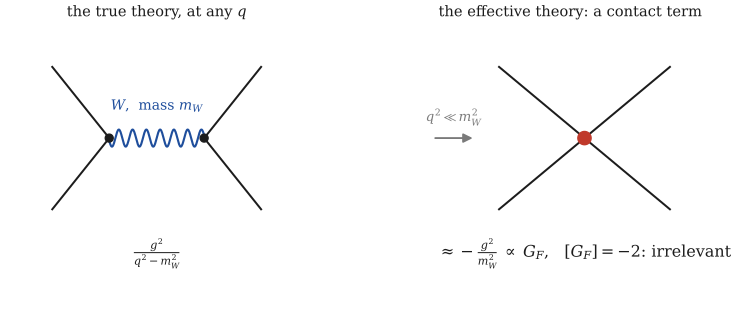
At energies far below \(m_W\), the \(W\) propagator \(g^2/(q^2-m_W^2)\) is basically a constant and the exchange looks like a point interaction. Fermi's theory is the full theory with the \(W\) integrated out: one step of Wilson's RG.
Integrating out the \(W\) gives \(\frac{G_F}{\sqrt2}=\frac{g^2}{8m_W^2}\). With the weak coupling \(g=0.652\) and \(m_W=80.377\) GeV, this gives \(G_F=1.163\times10^{-5}\ \mathrm{GeV}^{-2}\), within 0.3% of the measured value (loop corrections account for the rest). Fermi's theory wasn't wrong. It was the correct effective theory below \(m_W\), with its one number fixed by the physics above.
What "renormalisable" really means
Older textbooks treat renormalisability as a requirement: a sensible theory must only have couplings of zero or positive dimension. The Bogoliubov-Parasiuk-Hepp-Zimmermann (BPHZ) theorem sorts theories into three kinds:
super-renormalisable: every coupling has positive dimension (only finitely many diagrams diverge);
renormalisable: none has negative dimension (only finitely many kinds of infinity, so finitely many counterterms);
non-renormalisable: at least one has negative dimension (you would need infinitely many counterterms to remove the cutoff completely).
Part 2's formula \(D=d-\frac{d-2}2N+(d-4)V\) is where this comes from. The effective-theory view, which Melo's notes argue for carefully, changes the verdict on the last kind:
"Non-renormalisable theories have infinities that can't be removed." False. They need infinitely many counterterms, one per term in the Lagrangian, but only if you insist on \(\Lambda\to\infty\).
"Non-renormalisable theories can't predict anything." Only if you want them to work at every energy. At \(E\ll\Lambda\) you keep a few terms and predict to any fixed accuracy with finitely many numbers. Fermi's theory, the theory of pions and gravity at everyday energies all work this way.
"Renormalisable theories are fundamental." No. They're what any theory looks like far below its cutoff, because everything else is irrelevant. The Standard Model being renormalisable tells you its new-physics scale is far above what we've tested. It doesn't tell you there's no new physics.
Why high-energy physics is hard
Universality is wonderful if you care about long distances, because it lets you ignore the details. Tong points out that it's a curse if you care about short distances.
This is why reaching new physics usually needs higher energy, not just more precision and why an irrelevant coupling with a measurably large effect (like \(G_F\)) is such a valuable clue.
Can a theory work at every energy?
Can a theory be valid at all energies, so that the cutoff really can go to infinity? Run the RG backwards, towards short distances and ask where it goes (Melo, "The continuum limit").
Trivial. In \(\phi^4\) theory in four dimensions the coupling grows towards short distances and hits a Landau pole (Part 7). The only way to push the cutoff to infinity and keep the pole above it is to set the low-energy coupling to zero, which leaves a free theory. The same is believed of QED. Neither is a problem in practice, because the poles are at absurd energies (\(10^{277}\) GeV for QED with the electron alone). These are perfectly good effective theories.
Asymptotically free. In QCD the coupling shrinks to zero at short distances, heading into the Gaussian fixed point. That's a river with a source, so the theory makes sense at all energies. Proving this rigorously for Yang-Mills theory is one of the Clay Millennium Prize Problems.
Asymptotically safe. The source is an interacting fixed point. We met one in Part 6: in \(d<4\), a theory whose short-distance end is Wilson-Fisher. Weinberg's asymptotic safety idea asks whether gravity, whose Newton constant is irrelevant (\([G_N]=-2\)), could have such a fixed point in four dimensions. Nobody knows yet.
Naturalness: why relevant couplings are a puzzle
Irrelevant couplings are harmless because they shrink as you go to lower energies. Relevant ones do the opposite: they grow towards low energy, so a small relevant coupling at low energy needs very careful tuning at high energy. That's the hierarchy problem from exercise 1.4, now in RG language.
Apart from the vacuum energy, the Higgs mass term is the Standard Model's only relevant coupling and its quantum corrections grow like \(\Lambda^2\). For the Higgs to be light compared with a cutoff near the Planck scale, the bare parameter must cancel the loop to about thirty digits. You saw this yourself in the Part 2 widget. The cosmological constant, a coupling of dimension four, is even worse, off by about 120 powers of ten. Whether these are clues about new physics or just accidents is one of the big open questions. The RG doesn't answer it, but it's the reason it's a question at all.
Where to go next
You now know the core of the renormalisation group. Some directions from here:
The functional RG. Instead of following a few couplings, follow the whole potential or action as it flows. Melo's notes derive the "local potential approximation", an equation for \(V(\phi)\) that finds the Wilson-Fisher point directly in \(d=3\), with no \(\epsilon\) expansion. The modern version is the Wetterich equation.
Conformal field theory. A fixed point doesn't change when you zoom and usually it has an even bigger symmetry called conformal symmetry. That symmetry is so powerful that the conformal bootstrap pins down the 3D Ising exponents to six digits. That's where the \(\nu=0.629971\) in Part 6 comes from. Tong's §3.6 is a gentle first look.
Continuous symmetries. Magnets whose spins can point in any direction, the Mermin-Wagner theorem and the Kosterlitz-Thouless transition, where a whole line of fixed points appears: Tong's Chapter 4.
Gauge theories. The QCD beta function, including the ghost fields: Peskin §16.5 to §16.7.
Reading list
D. Tong, Statistical Field Theory, Cambridge lecture notes. The best free introduction to the magnet side (Parts 3 to 6 here) and the source of most of this course's intuition.
J. F. Melo, Introduction to Renormalisation, arXiv:1909.11099. Short and conceptual and the backbone of the field theory side here. It has one sign slip in its low-energy QED discussion (flagged in Part 7).
L.-F. Li, Introduction to Renormalization in Field Theory, arXiv:1208.4700. Short and concrete on counterterms, BPH subtraction and divergences inside divergences (used in Part 2).
D. V. Shirkov, "Fifty years of the renormalization group", CERN Courier (2001). The history, told by one of the people who built it.
M. E. Peskin and D. V. Schroeder, An Introduction to Quantum Field Theory: Ch. 6.3 (Wick rotation), Ch. 10 (infinities and counterterms) and Ch. 12 (Wilson, Callan-Symanzik, running).
A. Das, Field Theory: A Path Integral Approach, 3rd edition: Ch. 4 (Euclidean rotation), Ch. 10 (effective action and the loop expansion), Ch. 14 and 15 (critical exponents, the Ising model and duality).
M. Kardar, Statistical Physics of Fields, Ch. 3 to 5. The standard textbook version of Parts 4 to 6.
K. G. Wilson and J. Kogut, "The renormalization group and the ε expansion", Physics Reports 12 (1974) 75. Where it all started and still readable.
Exercises
Show solution
Show solution
Show solution