
Where Feynman diagrams come from
Where loop integrals come from
Why we rotate to Euclidean space
- Step 1: find the poles, rather than being told where they are
- Step 2: notice which quarters of the plane are empty
- Step 3: why you are allowed to rotate (the step usually skipped)
- Step 4: do the rotation, keeping every \(i\)
- A worked example, both ways
- What the rotation means, beyond the algebra
- Doing the rotation by computer
- Why this also joins QFT to statistical physics
Why loop integrals blow up
The cutoff and other ways to regularise
Doing a loop integral from start to finish
Same integral, three regulators
Renormalisation: trade the made-up numbers for measured ones
Hold the physics fixed and move the cutoff
- Exercises
Renormalisation Group II: Loops, Infinities and Cutoffs from Scratch
Part 2 of eight. previous: Why scale matters · Course home · Glossary · next: Block spins
Part 1 pulled Feynman rules out of thin air and used words like loop, Euclidean, cutoff and regularise without explaining them. This part builds all of it slowly, starting from the path integral itself: first where the diagrams and their rules come from, then why loops diverge, what a cutoff is and what renormalisation actually does. If you have Peskin & Schroeder or Ashok Das's Field Theory: A Path Integral Approach, the matching sections are mentioned as we go, but you don't need them.
Where Feynman diagrams come from
Where Feynman diagrams come from
Part 1 pulled three rules out of thin air: a line means \(1/(k^2+m^2)\), a vertex means \(\lambda_0/4!\) with a minus sign and a loop means "integrate over \(k\)". None of that was justified. Here is where all of it comes from, in one calculation.
Everything in this theory is an average over field shapes, weighted by \(e^{-S}\):
\[ \langle\,\cdots\rangle = \frac{\int\mathcal D\phi\;(\cdots)\;e^{-S_0[\phi]-S_{\rm int}[\phi]}}{\int\mathcal D\phi\;e^{-S_0[\phi]-S_{\rm int}[\phi]}},\qquad S_{\rm int}=\frac{\lambda_0}{4!}\int\mathrm d^dz\,\phi(z)^4. \]Two facts do all the work, both proved in Part 5:
Without the interaction, the average of two fields is the propagator: \(\langle\phi(x)\phi(y)\rangle_0=G(x-y)\), which in momentum space is \(1/(k^2+m^2)\). That's where the line comes from.
Wick's theorem: with the free weight, the average of any number of fields is the sum over all ways of pairing them up, each pair giving a propagator. Averages of an odd number vanish. To pair two fields, also called contracting them, means nothing more than taking those two out of the list and writing \(G\) for them. Part 5 derives the theorem in three lines from a source trick, so you never have to take it on faith.
Now expand the exponential, since \(\lambda_0\) is small:
\[ e^{-S_{\rm int}} = 1 - \frac{\lambda_0}{4!}\int\mathrm d^dz\,\phi(z)^4 + \dots \]Every vertex comes with a minus sign, simply because the exponential expands with alternating signs. That's the minus sign Part 1 used without explaining.
Take the two-point function \(\langle\phi(x)\phi(y)\rangle\) and keep the first-order term:
\[ -\frac{\lambda_0}{4!}\int\mathrm d^dz\;\big\langle\phi(x)\,\phi(y)\,\phi(z)\phi(z)\phi(z)\phi(z)\big\rangle_0 . \]Six fields, so Wick's theorem gives \(5\times3\times1=15\) pairings. Sort them into two kinds:
3 pairings join \(x\) straight to \(y\) and pair the four \(z\)'s among themselves. The diagram falls into two disconnected pieces and such pieces are exactly cancelled by the denominator of the average. Ignore them.
12 pairings connect everything: \(x\) pairs with one of the four \(\phi(z)\) (4 choices), \(y\) with one of the remaining three (3 choices) and the last two \(\phi(z)\) pair with each other (1 way). That's \(4\times3\times1=12\).
So the term is
\[ -\frac{\lambda_0}{4!}\cdot 12\int\mathrm d^dz\;G(x-z)\,G(z-y)\,G(0) = -\frac{\lambda_0}{2}\int\mathrm d^dz\;G(x-z)\,G(z-y)\,G(0). \]Look at what each piece became. The two propagators \(G(x-z)\) and \(G(z-y)\) are the particle travelling in and out. The factor \(G(0)=G(z-z)\) is a propagator that starts and ends at the same point: the loop. In momentum space a propagator at zero separation is
\[ G(0)=\int\frac{\mathrm d^dk}{(2\pi)^d}\,\frac{1}{k^2+m^2}, \]which is exactly the loop integral of Part 1. And the leftover number, \(12/4!=\tfrac12\), is Part 1's factor.
So the Feynman rules are not magic. A diagram is a bookkeeping picture for one group of Wick pairings: lines are propagators, dots are vertices from expanding \(e^{-S_{\rm int}}\) (each with a minus sign and a \(\lambda_0\)), closed loops are propagators that return to their own vertex and the symmetry factor counts how many pairings gave the same picture. Everything in Parts 1, 6 and 7 is this calculation, done for bigger diagrams.
Where loop integrals come from
Where loop integrals come from
Draw a Feynman diagram and at every dot (vertex) apply one rule: momentum in equals momentum out. For a diagram with no closed loops (a tree diagram), that rule fixes every internal momentum. Nothing is left to integrate.
Close a loop and something new happens. Momentum conservation at each dot still holds, but it no longer fixes everything:
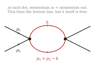
Two particles come in with \(p_1\) and \(p_2\). Momentum conservation fixes the bottom line once the top line's momentum \(k\) is chosen, but nothing fixes \(k\) itself.
Quantum mechanics says: when something isn't fixed, add up all the possibilities. So every loop comes with an integral over its free momentum,
\[ \int\frac{\mathrm d^4k}{(2\pi)^4}\,(\text{the propagators that depend on }k). \]The loop is a virtual particle that appears and disappears and \(k\) is its momentum. Because it's never observed, every value of \(k\) contributes, including huge ones. That word "every" is where the trouble in Part 1 came from.
One more useful fact: loops are the quantum part. If you keep track of \(\hbar\), a diagram with \(L\) loops carries an extra \(\hbar^{L}\) compared with the tree diagram with the same outside lines. Tree diagrams are classical physics and loops are the quantum jitter on top (Das §10.3).
Why we rotate to Euclidean space
Why we rotate to Euclidean space
In ordinary (Minkowski) spacetime, the propagator of a particle with mass \(m\) is
\[ \frac{i}{(k^0)^2-\mathbf k^2-m^2+i\varepsilon}. \]The tiny \(+i\varepsilon\) is Feynman's rule for which way particles go in time. Think of the integral over the energy \(k^0\) as a path along the real line in the complex \(k^0\) plane.
Step 1: find the poles, rather than being told where they are
The propagator blows up where its denominator vanishes. Set it to zero with \(E_k=\sqrt{\mathbf k^2+m^2}\):
\[ (k^0)^2 - E_k^2 + i\varepsilon = 0 \qquad\Longrightarrow\qquad k^0 = \pm\sqrt{E_k^2 - i\varepsilon}. \]Now expand the square root for small \(\varepsilon\), using \(\sqrt{a-x}\approx\sqrt a - \tfrac{x}{2\sqrt a}\):
\[ \sqrt{E_k^2 - i\varepsilon} \approx E_k - \frac{i\varepsilon}{2E_k}. \]So the two poles sit at
\[ k^0 = +E_k - \frac{i\varepsilon}{2E_k} \quad\text{(just \textit{below} the real axis, on the right)}, \qquad k^0 = -E_k + \frac{i\varepsilon}{2E_k} \quad\text{(just \textit{above} it, on the left)}. \]That is the whole content of the \(i\varepsilon\): it decides which side of the real axis each pole falls on. Nothing else in the calculation depends on it.
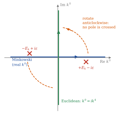
The two poles (red crosses) sit in the top-left and bottom-right quarters. The other two quarters are empty, so the blue path along the real line can be swung round onto the green imaginary line without touching a pole. (Peskin & Schroeder Fig. 6.1; Das Fig. 4.2.)
Step 2: notice which quarters of the plane are empty
Put those two poles on a picture. One is in the bottom-right quarter, the other in the top-left. The top-right with the bottom-left quarters contain nothing at all.
That is the fact the whole rotation rests on. If the \(i\varepsilon\) had the other sign, the poles would sit in the other two quarters, the free quarters would be different, so the rotation would have to go the other way.
Step 3: why you are allowed to rotate (the step usually skipped)
Cauchy's theorem says that the integral around a closed loop containing no poles is zero. Our path is not closed, so we have to build a closed one out of four pieces:
the real axis from \(-R\) to \(+R\), which is the integral we want,
a quarter-circle arc of radius \(R\) sweeping up through the empty top-right quarter,
the imaginary axis coming back down from \(iR\) to \(-iR\),
another quarter-circle through the empty bottom-left quarter.
No poles are enclosed, so those four pieces add to zero. That gives "real axis integral \(=\) imaginary axis integral" only if the two arcs contribute nothing. So check it, rather than hoping.
On the arc, \(|k^0| = R\). The integrand falls off like \(1/R^2\), since the denominator is dominated by \((k^0)^2\) when \(R\) is large. The length of a quarter-circle grows like \(R\). So the arc contributes at most about
\[ \frac{\pi R/2}{R^2 - E_k^2} \;\xrightarrow[R\to\infty]{}\; 0 . \]The arcs vanish. Now the rotation is justified.
Step 4: do the rotation, keeping every \(i\)
Set \(k^0 = ik^4\) with \(k^4\) real. Two things change, both of which must be tracked.
The measure. \(k^0 = ik^4\) gives \(\mathrm d k^0 = i\,\mathrm d k^4\). That factor of \(i\) is not optional, it travels with the integral for the rest of the calculation.
The invariant. \((k^0)^2 = (ik^4)^2 = -(k^4)^2\), so
\[ (k^0)^2 - \mathbf k^2 - m^2 \;=\; -(k^4)^2 - \mathbf k^2 - m^2 \;=\; -\big(k_E^2 + m^2\big), \qquad k_E^2 \equiv (k^4)^2 + \mathbf k^2 . \]This is the Wick rotation. Note what \(k_E^2\) is: a sum of four squares, so it is positive, while it treats the time direction exactly like the three space directions. Track the factors and the propagator becomes
\[ \frac{i}{k^2-m^2+i\varepsilon} \;\longrightarrow\; \frac{-i}{k_E^2+m^2}, \]whose \(-i\) then meets the \(i\) from the measure, so that the combination actually appearing under the integral, \(\mathrm d k^0\,i/(k^2-m^2+i\varepsilon)\), becomes the clean \(\mathrm d k^4/(k_E^2+m^2)\). Either way the useful part is the same: no poles anywhere on the real axis, no \(i\varepsilon\) left to worry about, because \(k_E^2+m^2\) never vanishes for real \(k_E\).
A worked example, both ways
Nothing above is convincing until you watch the two routes land on the same number. Take the simplest case, dropping the \(\mathbf k\) integral entirely and writing \(E\) for \(E_k\):
\[ I = \int_{-\infty}^{\infty}\frac{\mathrm d k^0}{(k^0)^2 - E^2 + i\varepsilon}. \]Route A, staying in Minkowski space and using residues. Keep \(\varepsilon\) finite for now, writing \(a = \sqrt{E^2 - i\varepsilon}\), so the denominator factorises cleanly as \((k^0-a)(k^0+a)\) with neither pole sitting on the path. This matters: a pole on the contour cannot simply be ignored, which is exactly what the \(i\varepsilon\) is there to prevent.
Close the contour with a big semicircle in the upper half plane. It contributes nothing, by the same \(1/R\) argument as in Step 3. The only pole inside is the left one, at \(k^0 = -a\), whose residue is
\[ \left.\frac{1}{k^0-a}\right|_{k^0=-a} = -\frac{1}{2a}. \]Cauchy's residue theorem gives \(2\pi i\) times that:
\[ I_\varepsilon = 2\pi i\cdot\left(-\frac{1}{2a}\right) = -\frac{i\pi}{a}. \]Only now let \(\varepsilon\to0^+\), so that \(a\to E\):
\[ I = -\frac{i\pi}{E}. \]Route B, rotating first. Substitute \(k^0 = ik^4\), so \(\mathrm d k^0 = i\,\mathrm d k^4\) and \((k^0)^2 - E^2 = -(k^4)^2 - E^2\):
\[ I = \int_{-\infty}^{\infty}\frac{i\,\mathrm d k^4}{-(k^4)^2 - E^2} = -i\int_{-\infty}^{\infty}\frac{\mathrm d k^4}{(k^4)^2 + E^2}. \]That last integral is one you already know, \(\int\mathrm d x/(x^2+a^2) = \pi/a\). So
\[ I = -i\cdot\frac{\pi}{E} = -\frac{i\pi}{E}. \]The same answer. Once the deformation has been justified, Route B needs no residues, no pole bookkeeping, no \(i\varepsilon\): just a substitution followed by a first-year integral. The pole bookkeeping did not disappear, it was spent once, in Steps 1 to 3, to earn the right to rotate. Afterwards every integral is an ordinary one, which is the entire reason anybody rotates.
Show solution
The standard integral is \(\int_{-\infty}^{\infty}\mathrm d x/(x^2+a^2)^2 = \pi/(2a^3)\), so the answer is \(i\pi/(2E^3)\).
Dimensions: the original integrand goes like \(1/(\text{energy})^4\) with one power of energy from \(\mathrm d k^0\), leaving \(1/(\text{energy})^3\). The answer has \(E^3\) downstairs, as required. Notice also that squaring flipped the overall sign compared with the first example, because the minus from the rotation was raised to an even power.
Two checks worth doing. Differentiating the first result with respect to \(E^2\) gives \(\partial_{E^2}(-i\pi/E) = i\pi/(2E^3)\), the same answer. And note that what was squared here is the denominator as written; squaring the full Feynman propagator \(i/(k^2-m^2+i\varepsilon)\) brings an extra \(i^2=-1\) along with it.
What the rotation means, beyond the algebra
There is a reason this trick keeps appearing in a course about magnets.
The quantum weight is \(e^{iS}\), an oscillating phase, which makes every integral a delicate business of cancellation. Under \(t \to -i\tau\), that phase turns into
\[ e^{iS} \;\longrightarrow\; e^{-S_E}, \]a real, decaying weight. But \(e^{-S_E}\) is a Boltzmann factor, exactly the object from Part 3 that gives a magnet its probability of sitting in some arrangement. So the rotation does not just make integrals easier. It is the precise statement of why a quantum field theory in \(d\) spacetime dimensions is the same mathematics as a statistical system in \(d\) space dimensions, which is the bridge this whole course walks across.
Doing the rotation by computer
You don't have to take Cauchy's word for it. Wolfram can do the complex integral directly, \(i\varepsilon\) and all:
(* 1. along the real k0 line, with the i eps kept *)
Integrate[1/(k0^2 - e^2 + I eps), {k0, -Infinity, Infinity}, Assumptions -> {e > 0, eps > 0}]
(* Pi/Sqrt[-e^2 + I eps]   ->   -I Pi/e  as eps -> 0 *)

(* 2. along the imaginary line, k0 = I k4, dk0 = I dk4 *)
Integrate[I/(-k4^2 - e^2), {k4, -Infinity, Infinity}, Assumptions -> e > 0]
(* -I Pi/e : the same *)

(* 3. where are the poles?  (e = 1, eps = 1/10) *)
k0 /. Solve[k0^2 - 1 + I/10 == 0, k0] // N
(* {-1.001 + 0.050 I, 1.001 - 0.050 I} : top-left and bottom-right, as in the picture *)

(* 4. a full 4D integral, done both ways (Peskin eq. 6.49) *)
inner = Integrate[1/(k0^2 - w^2 + I eps)^3, {k0, -Infinity, Infinity}, Assumptions -> {w > 0, eps > 0}];
inner0 = Limit[inner, eps -> 0, Direction -> "FromAbove"];                    (* -3 I Pi/(8 w^5) *)
Integrate[4 Pi p^2 (inner0 /. w -> Sqrt[p^2 + Dl]), {p, 0, Infinity}, Assumptions -> Dl > 0]/(2 Pi)^4
(* -I/(32 Pi^2 Dl) *)
(-1)^3 I 2 Pi^2 Integrate[k^3/(k^2 + Dl)^3, {k, 0, Infinity}, Assumptions -> Dl > 0]/(2 Pi)^4
(* -I/(32 Pi^2 Dl) : the Wick-rotated answer agrees *)
In the last check, the first calculation does the energy integral as a genuine contour integral in Minkowski space, then the three momentum integrals. The second does the whole thing as one rotated, four-dimensional Euclidean integral. They agree exactly. That's the Wick rotation, checked.
After the rotation we can use four-dimensional spherical coordinates, just as you use \(\mathrm d^3k = 4\pi k^2\,\mathrm d k\) in three dimensions:
\[ \int\mathrm d^4k_E = 2\pi^2\int_0^\infty k^3\,\mathrm d k, \]because the "surface area" of a unit sphere in four dimensions is \(2\pi^2\). In \(d\) dimensions it's \(S_d = 2\pi^{d/2}/\Gamma(d/2)\).
Why this also joins QFT to statistical physics
Rotating time the same way, \(\tau = it\), turns the quantum weight \(e^{iS}\) into \(e^{-S_E}\): a real, positive weight, just like the Boltzmann factor \(e^{-E/k_BT}\) of statistical mechanics.
This is why this course can move between magnets and particles so freely (Peskin §9.3, Das §14.1, Tong §2.3). From now on every momentum is Euclidean and I drop the \(E\).
Why loop integrals blow up
Why loop integrals blow up
Count the powers of \(k\). The tadpole from Part 1 has one loop and one propagator:
\[ \int\mathrm d^4k\,\frac{1}{k^2+m^2}\sim\int^{\infty}\frac{k^3\,\mathrm d k}{k^2} = \int^{\infty}k\,\mathrm d k \to\infty. \]At large \(k\) the measure gives four powers (\(k^3\,\mathrm d k\)) and the propagator takes away only two, so the integral grows like \(k^2\). We call that a quadratic divergence. The bubble in the picture above has two propagators, so it goes like \(\int k^3\mathrm d k/k^4=\int\mathrm d k/k\). That grows like \(\ln k\): a logarithmic divergence.
Peskin (§10.1) turns this counting into a rule. For a diagram with \(L\) loops and \(P\) internal lines, the superficial degree of divergence is
\[ D = (\text{powers of }k\text{ on top}) - (\text{powers on the bottom}) = 4L-2P. \]If \(D>0\) the integral diverges like \(\Lambda^D\), if \(D=0\) like \(\ln\Lambda\) and if \(D<0\) it usually converges. For \(\phi^4\) theory, use two facts. First, \(L=P-V+1\): each internal line brings a momentum, each of the \(V\) vertices imposes one conservation law and one of those laws is just overall conservation. Second, \(4V=N+2P\): each vertex has four legs, each internal line uses two and each of the \(N\) outside lines uses one. Eliminating \(L\) and \(P\) gives
\[ \boxed{\;D = 4-N.\;} \]This is a remarkable result. How badly a diagram diverges depends only on how many lines stick out of it, not on how complicated it is inside.
| outside lines \(N\) | \(D\) | what it corrects | how it diverges |
|---|---|---|---|
| 2 | 2 | the mass | like \(\Lambda^2\) |
| 4 | 0 | the coupling \(\lambda\) | like \(\ln\Lambda\) |
| 6, 8, ... | negative | nothing new | finite |
So in the whole theory, only two kinds of number ever blow up: the mass and the coupling. (The overall size of the field also needs a small fix, starting at two loops.) That short list is what "renormalisable" means and in Part 5 you'll see it's the same list as the couplings that survive coarse-graining.
The cutoff and other ways to regularise
The cutoff and other ways to regularise
To get a finite answer we must change the theory at very short distances, in a way controlled by one adjustable number. That step is called regularisation. Then we ask which predictions depend on the adjustable number and which don't.
Here are four common ways to do it.
A hard momentum cutoff. Only integrate up to \(|k|=\Lambda\). This is the easiest one to picture and it's the one Wilson's picture uses. Its weakness is that in gauge theories it breaks gauge symmetry, which is why particle physicists often prefer the next two.
A lattice. Put the field on a grid with spacing \(a\). Then no wave can be shorter than the grid allows, so \(\Lambda\sim\pi/a\). For a magnet this isn't a trick at all, because the atoms really do sit on a lattice. It's also how QCD is simulated on computers.
Pauli-Villars. Subtract the same diagram with an imaginary, very heavy particle of mass \(M\):
\[ \frac1{k^2+m^2}\to\frac1{k^2+m^2}-\frac1{k^2+M^2}=\frac{M^2-m^2}{(k^2+m^2)(k^2+M^2)}. \]For \(k\ll M\) nothing changes. For \(k\gg M\) the integrand falls off two powers faster, which is enough to make the bubble converge. Here \(M\) plays the role of \(\Lambda\).
Dimensional regularisation. The bubble diverges in four dimensions but converges in fewer, because there is less room (\(k^{d-1}\,\mathrm d k\)) at large \(k\). So do the integral in a general dimension \(d\), where the answer is a finite formula in \(d\) and only at the end let \(d\) approach 4. The infinity then shows up as a term like \(1/\epsilon\), with \(\epsilon=4-d\). For the tadpole:
\[ \int\frac{\mathrm d^dk}{(2\pi)^d}\,\frac1{k^2+m^2} = \frac{\Gamma(1-\tfrac d2)}{(4\pi)^{d/2}}\,(m^2)^{d/2-1}\ \xrightarrow{\ d=4-\epsilon\ }\ -\frac{m^2}{8\pi^2\epsilon}+\text{finite}. \]This method respects every symmetry and Part 7 uses it. The price is that it needs an arbitrary mass scale \(\mu\) to keep the units right in \(d\neq4\) and that \(\mu\) turns out to be where the "running" of couplings comes from.
Doing a loop integral from start to finish
Doing a loop integral from start to finish
Every one-loop integral in this course and almost every one in Peskin, is done with the same five-step recipe (Peskin §6.3 lists it right after computing the electron's magnetic moment):
Draw the diagram and write down the integral.
Use Feynman parameters to squeeze all the denominators into one.
Complete the square in that denominator by shifting the loop momentum.
Tidy up the numerator: throw away odd powers of the loop momentum and simplify even ones.
Wick rotate, use four-dimensional spherical coordinates and apply one master formula.
Let's do every step, with nothing skipped, on the bubble from the picture in section 2. We're already in Euclidean space, so the Wick rotation of step 5 is done.
Step 1: write the integral
With incoming momentum \(p=p_1+p_2\), the two lines of the loop carry \(k\) and \(k+p\), so the bubble is
\[ B(p) = \int\frac{\mathrm d^dk}{(2\pi)^d}\,\frac{1}{(k^2+m^2)\big((k+p)^2+m^2\big)}. \]We write \(d\) dimensions rather than 4 so we can use dimensional regularisation at the end.
Step 2: Feynman parameters
The trouble is that there are two different denominators, one centred on \(k=0\) and one on \(k=-p\), so the integrand has no simple symmetry. Feynman's trick squeezes them into one. For any two positive numbers \(A\) and \(B\),
\[ \frac{1}{AB} = \int_0^1\frac{\mathrm d x}{\big[xA+(1-x)B\big]^2}. \]Let's check it. The derivative of \(\dfrac{-1}{(A-B)\,[xA+(1-x)B]}\) with respect to \(x\) is \(\dfrac{1}{[xA+(1-x)B]^2}\), because the inside of the bracket has derivative \(A-B\). So the integral is that antiderivative at \(x=1\) minus its value at \(x=0\):
\[ \int_0^1\frac{\mathrm d x}{[xA+(1-x)B]^2} = \frac{-1}{(A-B)A}-\frac{-1}{(A-B)B} = \frac{-B+A}{(A-B)AB} = \frac{1}{AB}. \quad\checkmark \]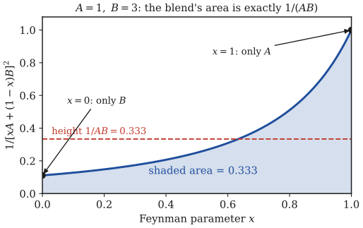
A Feynman parameter blends two denominators. At \(x=0\) you see only \(B\), at \(x=1\) only \(A\) and in between a mixture. The area under the blended curve is exactly \(1/AB\).
For three or more denominators the same idea works with more parameters (Peskin eq. 6.41):
\[ \frac{1}{A_1A_2\cdots A_n} = (n-1)!\int_0^1\mathrm d x_1\cdots\mathrm d x_n\,\delta\Big(\sum x_i-1\Big)\,\frac{1}{\big[x_1A_1+\dots+x_nA_n\big]^n}. \]The delta function just says the mixture fractions add up to one. (Checked in Wolfram for \(n=3\).)
For our bubble, take \(A=(k+p)^2+m^2\) and \(B=k^2+m^2\):
\[ B(p) = \int_0^1\mathrm d x\int\frac{\mathrm d^dk}{(2\pi)^d}\,\frac{1}{\big[x\big((k+p)^2+m^2\big)+(1-x)\big(k^2+m^2\big)\big]^2}. \]Step 3: complete the square
Multiply out the square bracket. The \(k^2\) and \(m^2\) terms appear with total weight \(x+(1-x)=1\) and \((k+p)^2=k^2+2k\cdot p+p^2\), so
\[ x\big((k+p)^2+m^2\big)+(1-x)\big(k^2+m^2\big) = k^2 + 2x\,k\cdot p + x\,p^2 + m^2. \]Now complete the square, exactly as you would for \(k^2+2bk\): \(\;k^2+2x\,k\cdot p = (k+xp)^2 - x^2p^2\). So
\[ k^2 + 2x\,k\cdot p + x\,p^2 + m^2 = (k+xp)^2 + x(1-x)\,p^2 + m^2. \]Define the shifted loop momentum \(\ell = k+xp\) and the constant
\[ \Delta = m^2 + x(1-x)\,p^2. \]The denominator is now just \((\ell^2+\Delta)^2\). Shifting the integration variable doesn't change the integral, since \(\mathrm d^d k=\mathrm d^d\ell\) and both run over all of space:
\[ B(p) = \int_0^1\mathrm d x\int\frac{\mathrm d^d\ell}{(2\pi)^d}\,\frac{1}{(\ell^2+\Delta)^2}. \]Step 4: tidy up the numerator
Here the numerator is just \(1\), so there's nothing to do. In QED (Part 7) the numerator contains \(\ell^\mu\) and \(\ell^\mu\ell^\nu\), so two rules are needed:
\[ \int\frac{\mathrm d^d\ell}{(2\pi)^d}\,\frac{\ell^\mu}{D^3} = 0, \qquad \int\frac{\mathrm d^d\ell}{(2\pi)^d}\,\frac{\ell^\mu\ell^\nu}{D^3} = \frac{g^{\mu\nu}}{d}\int\frac{\mathrm d^d\ell}{(2\pi)^d}\,\frac{\ell^2}{D^3}. \]These are Peskin's equations 6.45 and 6.46. They get quoted as "by symmetry" far too quickly, so here is where they come from. Everything rests on one fact established in Step 3: after the shift, \(D\) depends only on \(\ell^2\), never on the direction of \(\ell\).
Two pieces of small print before we start. First, the argument below is cleanest after the Wick rotation of section 3, where all \(d\) directions really are alike and the natural object is the Euclidean \(\delta^{ab}\); the covariant statement with \(g^{\mu\nu}\) follows from it. Second, it assumes the integral is defined, which for the rank-two case at \(d=4\) means dimensionally regularised, since that integral is logarithmically divergent. A regulator that respects the symmetry is what lets you shuffle the integrand this way at all.
The first rule. Send \(\ell \to -\ell\). The measure \(\mathrm d^d\ell\) is unchanged, since flipping every axis is just a relabelling. \(D\) is unchanged, because it only knows \(\ell^2\). The numerator \(\ell^\mu\) flips sign. So the whole integral equals minus itself:
\[ I^\mu = -I^\mu \qquad\Longrightarrow\qquad I^\mu = 0. \]Nothing deeper than that. For every \(\ell\) contributing \(+3\), the point \(-\ell\) contributes \(-3\).
The second rule, the one that looks like magic. Take it in two pieces.
Off the diagonal, say \(\mu = 1\) with \(\nu = 2\). Now flip only the second axis, \(\ell^2 \to -\ell^2\), leaving the rest alone. Again the measure and \(D\) do not notice, because \(D\) depends on the length. The numerator \(\ell^1\ell^2\) flips sign. Same argument as before, so every off-diagonal component vanishes.
On the diagonal, the components cannot be calculated one at a time, but they do not need to be, because in Euclidean space they are all equal. Nothing in the integral distinguishes one axis from another: the only thing \(D\) knows is the length of \(\ell\), which treats every direction alike. So whatever number \(\int \ell^1\ell^1/D^3\) comes to, \(\int\ell^2\ell^2/D^3\) comes to the same. That holds for all \(d\) of them.
Put those together. The answer is zero off the diagonal, with \(d\) equal entries on it, which in Euclidean space is precisely the statement that it is proportional to \(\delta^{ab}\). Rotating back, the covariant version reads
\[ \int\frac{\mathrm d^d\ell}{(2\pi)^d}\frac{\ell^\mu\ell^\nu}{D^3} = A\,g^{\mu\nu}\quad\text{for some number }A. \](Note that the Minkowski \(g^{\mu\nu}\) does not have \(d\) equal diagonal entries, since its time entry has the opposite sign. The "all directions alike" step is the Euclidean one. What survives the rotation is the statement that no vector is available to build the answer from, leaving the metric as the only rank-two object in sight.)
Finding \(A\) takes one line. Contract both sides with \(g_{\mu\nu}\). On the left, \(g_{\mu\nu}\ell^\mu\ell^\nu = \ell^2\). On the right, \(g_{\mu\nu}g^{\mu\nu} = g^\mu{}_\mu = d\), the trace of the identity in \(d\) dimensions rather than of the metric. So
\[ \int\frac{\mathrm d^d\ell}{(2\pi)^d}\frac{\ell^2}{D^3} = A\,d \qquad\Longrightarrow\qquad A = \frac1d\int\frac{\mathrm d^d\ell}{(2\pi)^d}\frac{\ell^2}{D^3}, \]which is the rule. The \(1/d\) is not a convention or a fudge. It is there because the trace of the metric is \(d\), so the one number \(A\) has to be shared out over \(d\) equal diagonal entries.
Show solution
For the off-diagonal piece, \(\int \ell_x\ell_y f = G_1\,G_1\,G_0 = 0\), since each odd integral vanishes on its own.
For the diagonal, \(\int\ell_x^2 f = G_2\,G_0\,G_0 = \tfrac{\sqrt\pi}{2}\pi = \tfrac{\pi^{3/2}}{2}\). By the same computation \(\int\ell_y^2f\) and \(\int\ell_z^2f\) give the identical number, so
\[ \int \ell^2 f = \int(\ell_x^2+\ell_y^2+\ell_z^2)f = 3\times\frac{\pi^{3/2}}{2}, \]and therefore \(\int\ell_x^2 f = \tfrac13\int\ell^2f\) exactly. The \(3\) appeared for the reason given above: three equal contributions sharing one total.
Step 5: spherical coordinates and the master formula
In \(d\) dimensions, \(\mathrm d^d\ell = S_d\,\ell^{d-1}\mathrm d\ell\), where \(S_d=2\pi^{d/2}/\Gamma(d/2)\) is the area of the unit sphere (this is \(2\pi^2\) for \(d=4\)). So
\[ \int\frac{\mathrm d^d\ell}{(2\pi)^d}\,\frac{1}{(\ell^2+\Delta)^n} = \frac{S_d}{(2\pi)^d}\int_0^\infty\frac{\ell^{d-1}\,\mathrm d\ell}{(\ell^2+\Delta)^n}. \]Substitute \(t=\ell^2/\Delta\), so \(\ell=\sqrt{\Delta t}\) and \(\mathrm d\ell = \frac{\sqrt\Delta}{2\sqrt t}\,\mathrm d t\). The radial integral becomes
\[ \int_0^\infty\frac{\ell^{d-1}\,\mathrm d\ell}{(\ell^2+\Delta)^n} = \frac12\,\Delta^{d/2-n}\int_0^\infty\frac{t^{d/2-1}\,\mathrm d t}{(1+t)^n} = \frac12\,\Delta^{d/2-n}\,\frac{\Gamma(\tfrac d2)\,\Gamma(n-\tfrac d2)}{\Gamma(n)}. \]The last step uses a standard integral, \(\int_0^\infty t^{a-1}(1+t)^{-a-b}\,\mathrm d t=\Gamma(a)\Gamma(b)/\Gamma(a+b)\) (the "beta function"). Multiply by \(S_d/(2\pi)^d = 2/\big((4\pi)^{d/2}\Gamma(d/2)\big)\) and the \(\Gamma(d/2)\) and the \(2\) cancel:
\[ \boxed{\;\int\frac{\mathrm d^d\ell}{(2\pi)^d}\,\frac{1}{(\ell^2+\Delta)^n} = \frac{\Gamma(n-\tfrac d2)}{(4\pi)^{d/2}\,\Gamma(n)}\;\Delta^{d/2-n}.\;} \]This is the master formula. Every one-loop integral in the course is a special case. With \(n=1\) it's the tadpole formula of section 5. With \(n=2\) it gives our bubble:
\[ B(p) = \frac{\Gamma(2-\tfrac d2)}{(4\pi)^{d/2}}\int_0^1\mathrm d x\;\Delta^{d/2-2}. \]Step 6: let \(d\) approach 4
Put \(d=4-\epsilon\), so \(2-\tfrac d2 = \tfrac\epsilon2\). There are three factors to expand, keeping terms up to \(\epsilon^0\):
\(\Gamma(\tfrac\epsilon2) = \tfrac2\epsilon-\gamma_E+O(\epsilon)\), where \(\gamma_E=0.5772\dots\) is Euler's constant. The Gamma function has a pole at zero and this is where the infinity lives.
\((4\pi)^{-d/2} = (4\pi)^{-2}(4\pi)^{\epsilon/2} = \frac1{16\pi^2}\big(1+\tfrac\epsilon2\ln4\pi+\dots\big)\), using \(a^{\epsilon}=e^{\epsilon\ln a}\approx1+\epsilon\ln a\).
\(\Delta^{-\epsilon/2} = 1-\tfrac\epsilon2\ln\Delta+\dots\), the same trick.
Multiply the three. The \(\tfrac2\epsilon\) from the first factor times the \(\tfrac\epsilon2\) terms of the others gives finite pieces, so
\[ \boxed{\;B(p) = \frac{1}{16\pi^2}\left[\frac2\epsilon - \gamma_E + \ln4\pi - \int_0^1\mathrm d x\,\ln\big(m^2+x(1-x)p^2\big)\right]+O(\epsilon).\;} \](Strictly, the logarithm is \(\ln(\Delta/\mu^2)\), with the scale \(\mu\) from section 5 keeping the units right.) The infinity is the \(2/\epsilon\). Everything that depends on the physics, meaning the masses and momenta, sits in the finite logarithm. Every step above was checked in Wolfram:
Integrate[1/(x A + (1 - x) B)^2, {x, 0, 1}, Assumptions -> {A > 0, B > 0}]     (* 1/(A B) *)
Expand[x ((k + p)^2 + m^2) + (1 - x) (k^2 + m^2) /. k -> l - x p]            (* l^2 + m^2 + x(1-x)p^2 *)
Sd = 2 Pi^(d/2)/Gamma[d/2];
Sd/(2 Pi)^d Integrate[l^(d - 1)/(l^2 + D0)^n, {l, 0, Infinity},
    Assumptions -> {D0 > 0, n > d/2, d > 0}] // FullSimplify
(* Gamma[n - d/2] D0^(d/2 - n)/((4 Pi)^(d/2) Gamma[n]) : the master formula *)
Series[Gamma[eps/2] (4 Pi)^(-(4 - eps)/2) D0^(-eps/2), {eps, 0, 0}]
(* (2/eps - EulerGamma + Log[4 Pi] - Log[D0])/(16 Pi^2) *)
Peskin's §6.3 uses exactly these steps on a harder integral, the correction to the electron's magnetic moment and ends with Schwinger's famous result \(\frac{g-2}{2}=\frac{\alpha}{2\pi}\approx0.0011614\) (exercise 2.6). Part 7 uses them on the QED vacuum polarisation.
Same integral, three regulators
Same integral, three regulators
This is the key lesson of the page, done with real numbers. Take the log-divergent bubble with no momentum flowing in,
\[ I(m) = \int\frac{\mathrm d^4k}{(2\pi)^4}\,\frac1{(k^2+m^2)^2}, \]and regularise it three different ways. (This is the bubble \(B(p)\) of section 6 at \(p=0\), so the dimensional-regularisation line is just section 5's answer with \(\Delta=m^2\).) Each was done symbolically in Wolfram:
\[ \begin{aligned} \text{cutoff:}&\quad I = \frac1{16\pi^2}\left[\ln\!\Big(1+\frac{\Lambda^2}{m^2}\Big)-\frac{\Lambda^2}{\Lambda^2+m^2}\right]\ \xrightarrow{\Lambda\gg m}\ \frac1{16\pi^2}\left[\ln\frac{\Lambda^2}{m^2}-1\right]\\ \text{Pauli-Villars:}&\quad I = \frac1{16\pi^2}\ln\frac{M^2}{m^2}\\ \text{dimensional:}&\quad I = \frac1{16\pi^2}\left[\frac2\epsilon-\gamma_E+\ln4\pi-\ln\frac{m^2}{\mu^2}\right] \end{aligned} \]Each one is infinite when its regulator is removed. But look at how each depends on \(m\). Every one contains \(-\frac1{16\pi^2}\ln m^2\), plus a constant that depends on the regulator but not on \(m\). So a difference such as \(I(m_1)-I(m_2)=\frac1{16\pi^2}\ln\frac{m_2^2}{m_1^2}\) comes out finite and it's the same in all three.
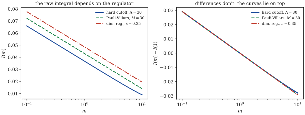
Left: the raw integral in the three methods differs by a constant shift and each shift grows without limit as its regulator is removed. Right: subtract the value at one reference mass and the three curves land on top of each other. (The cutoff curve bends away a little at the far right, where \(m\) is no longer much smaller than \(\Lambda=30\).)
ang = 2 Pi^2/(2 Pi)^4;                                   (* Vol(S^3)/(2Pi)^4 *)
Icut = ang Integrate[k^3/(k^2 + m^2)^2, {k, 0, L}, Assumptions -> {m > 0, L > 0}];
Ipv  = ang Integrate[k^3 (1/(k^2 + m^2)^2 - 1/(k^2 + M^2)^2), {k, 0, Infinity},
                     Assumptions -> {m > 0, M > m}];     (* Log[M^2/m^2]/(16 Pi^2) *)
Idr  = Gamma[2 - d/2]/(4 Pi)^(d/2) (m^2)^(d/2 - 2) mu^(4 - d);
Series[Idr /. d -> 4 - eps, {eps, 0, 0}]                 (* 2/eps - EulerGamma + ... *)
(* all three give dI/d(m^2) = -1/(16 Pi^2 m^2) once the regulator is large *)
That's the whole trick of renormalisation. The part that depends on the regulator is a constant and a constant can be soaked up into a number we never measure directly.
Renormalisation: trade the made-up numbers for measured ones
Renormalisation: trade the made-up numbers for measured ones
The numbers \(m_0\) and \(\lambda_0\) written in the Lagrangian are called bare parameters. Nobody measures them. What you measure is, for example, the position of the pole in the propagator (\(m_{\rm phys}\)) and a collision rate at some energy (which defines \(\lambda_{\rm phys}\)). Loops connect the two:
\[ m^2_{\rm phys} = m_0^2 + \delta m^2(\Lambda), \qquad \lambda_{\rm phys} = \lambda_0 + \delta\lambda(\Lambda). \]Ling-Fong Li's lecture notes (arXiv:1208.4700) point out that renormalisation isn't special to particle physics. An electron moving through a crystal responds to forces as if it had an effective mass \(m^*\), different from its mass \(m\) in empty space, because it's constantly tugging on the lattice. In a crystal, both \(m\) and \(m^*\) can be measured, since you can take the electron out. Quantum field theory differs in two ways: the shift from bare to physical is infinite (it comes from the high-momentum modes) and you can never switch the interactions off, so the bare value is never measurable.
The recipe has four steps:
Regularise, so every quantity is finite and depends on \(\Lambda\).
Work out the measured quantities in terms of the bare ones.
Turn that around: write the bare parameters in terms of the measured ones.
Rewrite every other prediction using the measured parameters.
After step 4, the \(\Lambda\) drops out of every prediction, at least in a renormalisable theory like \(\phi^4\) (Peskin §10.2 does this in full). The infinity hasn't been hidden under the carpet. It has been moved into the link between two sets of numbers and only one of those sets is ever measured.
Dmitry Shirkov, one of the founders of the renormalisation group, put it simply in his fifty-year retrospective in the CERN Courier: physical quantities come out as finite functions of the new "renormalised" couplings, with "all infinities being swallowed by the Z factors". The Z factors are the numbers that connect bare and renormalised quantities, such as \(m_0^2=Z_m m^2\).
Why only a few numbers ever need fixing
Here's a lovely fact from Li's notes that explains why renormalisation only needs a few counterterms. Take the bubble from section 6 and differentiate it with respect to the outside momentum. Each derivative puts one more power of the loop momentum in the denominator, so the integral becomes more convergent. Using section 5's formula,
\[ \frac{\partial B}{\partial p^2} = \frac{\Gamma(2-\tfrac d2)\,(\tfrac d2-2)}{(4\pi)^{d/2}}\int_0^1\mathrm d x\;x(1-x)\,\Delta^{d/2-3}. \]Now \(\Gamma(2-\tfrac d2)(\tfrac d2-2) = -\Gamma(3-\tfrac d2)\) and \(\Gamma(3-\tfrac d2)\to\Gamma(1)=1\) as \(d\to4\). So there's no pole left:
\[ \frac{\partial B}{\partial p^2} \xrightarrow{\ d\to4\ } -\frac{1}{16\pi^2}\int_0^1\frac{x(1-x)\,\mathrm d x}{m^2+x(1-x)p^2}\qquad\text{(finite).} \]So the infinity in \(B(p)\) lives entirely in its value at one point, \(B(0)\) and the difference \(B(p)-B(0)\) is finite. (Checked in Wolfram.) In general, an integral that diverges like \(\Lambda^D\) only has infinities in the first few terms of its Taylor series in the outside momenta, up to power \(D\). That's why a finite number of counterterms, one for each of those first few terms, is enough.
Counterterms as extra Feynman rules
There's a tidy way to organise all this, called renormalised perturbation theory (Li §2.2, Peskin §10.2). Write the Lagrangian in terms of the measured mass \(m\) and coupling \(\lambda\) and move everything that absorbs infinities into separate counterterms:
\[ \mathcal L = \underbrace{\tfrac12(\partial\phi)^2+\tfrac12m^2\phi^2+\frac{\lambda}{4!}\phi^4}_{\text{same form, measured numbers}} \;+\; \underbrace{\tfrac12\delta_Z(\partial\phi)^2+\tfrac12\delta_m\phi^2+\frac{\delta_\lambda}{4!}\phi^4}_{\text{counterterms}}. \]The counterterms are treated just like new interactions, with their own Feynman rules. They are drawn as a circle with a cross:
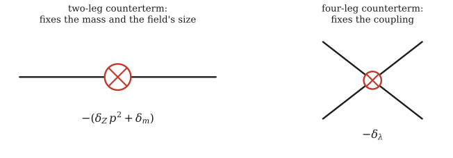
The two new vertices. The two-leg one fixes the mass and the size of the field; the four-leg one fixes the coupling. The numbers \(\delta_Z,\delta_m,\delta_\lambda\) are chosen, order by order, to cancel the infinities of the loop diagrams.
Beyond one loop
At two loops something new happens: a diagram can contain a smaller divergent diagram inside it. Take two bubbles in a row, a four-point diagram proportional to \(\lambda^3\Gamma(p)^2\), where \(\Gamma(p)\) is one bubble (Li's Fig. 9). Its overall degree of divergence is \(D=4-4=0\), which suggests one derivative should make it finite. But it doesn't, because each bubble diverges on its own and a derivative only helps one of them at a time.
The rescue comes from the one-loop counterterm. In the two-loop calculation, the counterterm vertex can replace either of the two bubbles:
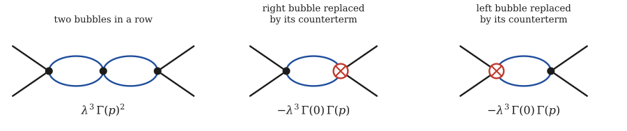
The two-loop chain and its two counterterm partners. Each partner contains one real bubble and one counterterm, which is worth \(-\Gamma(0)\).
Add the three together and complete the square:
\[ \lambda^3\,\Gamma(p)^2 - 2\lambda^3\,\Gamma(0)\,\Gamma(p) = \lambda^3\big[\Gamma(p)-\Gamma(0)\big]^2 - \lambda^3\,\Gamma(0)^2. \]The bracket is finite (that's the difference \(B(p)-B(0)\) from above) and the last term doesn't depend on \(p\) at all, so a new two-loop counterterm cancels it. So with the lower-order counterterms included, the leftover infinities are again just constants, the first term of a Taylor series and the same trick works at every order. This is the BPH recipe (Bogoliubov, Parasiuk and Hepp, later completed by Zimmermann):
Build the diagrams from the renormalised Lagrangian.
At one loop, find the infinite first Taylor terms and add counterterms to cancel them.
At two loops, include diagrams with the one-loop counterterms inside, then add new counterterms for what's left. Repeat at every order.
Divergences inside divergences can also be nested, one completely inside the other:
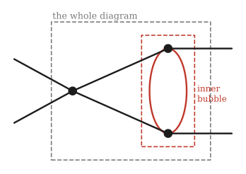
A nested divergence (Li's Fig. 11). The inner bubble diverges on its own and so does the whole diagram. The one-loop counterterm cures the inside and then a new two-loop counterterm cures the outside.
The rule that says when a multi-loop integral really converges is Weinberg's theorem: the whole diagram and every sub-diagram inside it must have negative degree of divergence. Proving that BPH always works is famously hard and Li's notes and Peskin §10.4 go further if you're curious. The takeaway for this course is simple: in a renormalisable theory, a finite list of counterterms, fixed order by order, removes every infinity.
Hold the physics fixed and move the cutoff
Hold the physics fixed and move the cutoff
Keep \(m_{\rm phys}\) and \(\lambda_{\rm phys}\) fixed, since those are what experiments tell you and ask what the bare parameters must be for different cutoffs. From Part 1,
\[ m_0^2(\Lambda) = m^2_{\rm phys}-\frac{\lambda}{32\pi^2}\left[\Lambda^2-m^2\ln\!\Big(1+\frac{\Lambda^2}{m^2}\Big)\right]. \]The bare coupling has to change with \(\Lambda\) too, only much more slowly, like a logarithm (Part 7 works out exactly how). The bare parameters are functions of the cutoff, arranged so that low-energy physics never notices the cutoff. That sentence is the renormalisation group. Wilson's big step, in Parts 5 and 6, was to take it literally and ask what happens when you lower \(\Lambda\) bit by bit.
Slide the cutoff up to the Planck scale (\(\log_{10}\Lambda\approx19\)) with a mass of 125 GeV, like the Higgs. The bare mass has to cancel the loop correction to about thirty digits. That's the "hierarchy problem" from exercise 1.4 and Part 8 explains why mass terms and only mass terms, are this sensitive.
Exercises
Show solution
Show solution
Show solution
Show solution
Show solution