
Renormalisation Group VII: Running Couplings
Part 7 of eight. previous: The Wilson-Fisher point · Course home · Glossary · next: Effective field theory
So far we have coarse-grained: we lowered a cutoff and watched the couplings flow. Particle physicists usually do it another way. They remove the cutoff completely (using dimensional regularisation from Part 2) and they fix the theory with a measurement made at some energy \(\mu\) that they choose. Then they ask how the answer depends on that choice. The result is the same kind of flow, now called the running of couplings with energy. This part shows that the two pictures agree and then applies the particle-physics version to QED and QCD, where the running has actually been measured.
Two questions, one idea
Books often blur these together, so it pays to be exact. Melo's notes separate two questions:
Wilson's question: keep the long-distance physics fixed. How must the bare couplings change as I move the cutoff \(\Lambda\)? That was Parts 5 and 6.
The particle physicist's question: keep the underlying theory fixed. How does the measured coupling depend on the energy \(\mu\) at which I measure it? That's this part.
Minimal subtraction, on one page
Work in \(d=4-\epsilon\) dimensions (Part 2). There the bare coupling \(\lambda_0\) has mass dimension \(\epsilon\), so to keep a pure-number coupling we bring in an arbitrary mass scale \(\mu\) and write
\[ \lambda_0 = \mu^{\epsilon}\left(\lambda + \frac{a_1(\lambda)}{\epsilon} + \frac{a_2(\lambda)}{\epsilon^2}+\dots\right). \]Here \(\lambda\) is the renormalised coupling at scale \(\mu\). The extra \(a_i/\epsilon\) terms are called counterterms. They're chosen to cancel the \(1/\epsilon\) infinities of the loop diagrams and do nothing else, which is why this scheme is called minimal subtraction (MS).
Now the key point. \(\lambda_0\) belongs to the actual theory and it cannot know about \(\mu\), which is a scale we made up. So \(\mu\,\mathrm d\lambda_0/\mathrm d\mu=0\).
Here's how that turns into a formula, step by step. Define \(\beta(\lambda)\equiv\mu\,\mathrm d\lambda/\mathrm d\mu\). Differentiate \(\lambda_0\) with respect to \(\mu\) using the product rule and the chain rule (\(a_1\) depends on \(\mu\) only through \(\lambda\)):
\[ 0 = \mu\frac{\mathrm d\lambda_0}{\mathrm d\mu} = \mu^\epsilon\left[\epsilon\Big(\lambda+\frac{a_1}{\epsilon}\Big) + \Big(1+\frac{a_1'}{\epsilon}\Big)\beta\right]+\dots, \]where \(a_1'=\mathrm d a_1/\mathrm d\lambda\). Divide by \(\mu^\epsilon\) and look for a \(\beta\) of the form \(\beta=-\epsilon\lambda+b(\lambda)\). Substituting it in and sorting by powers of \(\epsilon\):
the terms with \(\epsilon^1\): \(\;\epsilon\lambda-\epsilon\lambda = 0\), fine;
the terms with \(\epsilon^0\): \(\;a_1 + b - \lambda a_1' = 0\), so \(b=\lambda a_1'-a_1\);
the terms with \(1/\epsilon\) only involve higher loops and \(a_2\), so we can ignore them at one loop.
So
\[ \boxed{\;\beta(\lambda) = -\epsilon\lambda + \Big(\lambda\frac{\mathrm d}{\mathrm d\lambda}-1\Big)a_1(\lambda).\;} \](For a coupling written as \(g_0=\mu^{\rho\epsilon}(g+a_1/\epsilon+\dots)\) the same steps give \(\beta=-\rho\epsilon g+\rho\,(g\,a_1'-a_1)\). QED has \(\rho=\tfrac12\); see exercise 7.1.) So only the number in front of the simplest \(1/\epsilon\) matters. All of the running comes from the \(1/\epsilon\) of one-loop diagrams.
φ⁴: the bubble finds the Wilson-Fisher point again
Write \(\Gamma^{(4)}\) for the full strength of the four-particle interaction: the tree-level \(\lambda_0\) plus its loop corrections. (It is what you would measure in a collision of two particles into two.) At one loop it gets the bubble diagram of Part 2 in three different ways, called channels. The four outside legs can be paired up as (1,2) meeting (3,4), or (1,3) meeting (2,4), or (1,4) meeting (2,3) and the squared momentum flowing through the bubble in each case is called \(s\), \(t\) and \(u\) respectively. Taking particles 1 with 2 as incoming while 3 with 4 go out, those momenta are \(s=(p_1+p_2)^2\), \(t=(p_1-p_3)^2\) and \(u=(p_1-p_4)^2\). (Books that write every momentum as incoming flip the signs of the last two. Both conventions give \(s+t+u=\sum_i m_i^2\).) Each comes with a symmetry factor \(\tfrac12\):
\[ \Gamma^{(4)} = \lambda_0 - \frac{\lambda_0^2}{2}\big[B(s)+B(t)+B(u)\big]+\dots,\qquad B(p)=\int\frac{\mathrm d^dk}{(2\pi)^d}\frac1{(k^2+m^2)((k+p)^2+m^2)}. \]We computed exactly this integral, step by step, in Part 2, section 6 (Feynman parameter, completing the square, master formula, then \(d\to4\)):
\[ B(p) = \frac{\Gamma(2-\tfrac d2)}{(4\pi)^{d/2}}\int_0^1\mathrm d x\,\big[m^2+x(1-x)p^2\big]^{d/2-2} = \frac{1}{16\pi^2}\left[\frac2\epsilon+\text{finite}\right]. \](A warning about letters: this \(u\) is a momentum variable, nothing to do with the coupling \(\tilde u\) of Parts 5 and 6. Both names are too standard to change.) The three channels give an infinite part \(-\frac{\lambda^2}{2}\cdot3\cdot\frac{2}{16\pi^2\epsilon}=-\frac{3\lambda^2}{16\pi^2\epsilon}\). The counterterm must cancel it, so \(a_1=\frac{3\lambda^2}{16\pi^2}\) and
\[ \boxed{\;\beta(\lambda) = -\epsilon\lambda + \frac{3\lambda^2}{16\pi^2}.\;} \]Now compare with Part 6. There we integrated out shells of fast momentum modes and found a fixed point at \(\tilde u^*=16\pi^2\epsilon/3\). Here, setting \(\beta=0\):
\[ \lambda^* = \frac{16\pi^2}{3}\,\epsilon. \]The same number, from a completely different calculation. One used a hard cutoff and zooming out. The other used dimensional regularisation and a made-up scale \(\mu\), with no cutoff at all. The slope here, \(\beta'(\lambda^*)=+\epsilon\), is Part 6's \(-\epsilon\) read with RG time running the other way. Both were checked in Wolfram:
beta0[a1_, g_, rho_] := rho (g D[a1, g] - a1);             (* MS beta from the simple pole *)
Simplify[beta0[3 lam^2/(16 Pi^2), lam, 1]]                   (* 3 lam^2/(16 Pi^2) *)
I2 = Gamma[2 - d/2]/(4 Pi)^(d/2) (m^2 + x (1 - x) p^2)^(d/2 - 2);
Series[I2 /. d -> 4 - eps, {eps, 0, 0}]                      (* (1/(16 Pi^2)) (2/eps + ...) *)
beta = -eps lam + 3 lam^2/(16 Pi^2);
lam /. Last[Solve[beta == 0, lam]]                           (* 16 Pi^2 eps/3, same as Wilson *)
The \(\tfrac32\) we counted by hand in Part 6 (72 ways to join the lines) equals the \(3\times\tfrac12\) here (three channels, each with a factor of one half). Two independent calculations that had to agree and do.
The Callan-Symanzik equation
A real, measurable correlation function can't depend on the \(\mu\) we picked. Written in terms of \(\lambda(\mu)\), that simple fact becomes a differential equation, the Callan-Symanzik equation (Peskin §12.2):
\[ \Big[\mu\frac{\partial}{\partial\mu}+\beta(\lambda)\frac{\partial}{\partial\lambda}+n\,\gamma(\lambda)\Big]G^{(n)}(p_i;\lambda,\mu)=0. \]Here \(\gamma\) is the anomalous dimension of the field: how much its scaling differs from what plain dimensional analysis says. For \(\phi^4\), \(\gamma\) first appears at two loops, which is why \(\eta=\epsilon^2/54\) in Part 6. The equation just says that moving \(\mu\) can be exactly undone by moving \(\lambda\) (and rescaling the field).
Solving the flow: running and the Landau pole
In \(d=4\) the equation is \(\mu\,\mathrm d\lambda/\mathrm d\mu=3\lambda^2/16\pi^2\). Write \(L=\ln\mu\), so \(\mu\,\mathrm d/\mathrm d\mu=\mathrm d/\mathrm d L\) and separate the variables:
\[ \frac{\mathrm d\lambda}{\lambda^2} = \frac{3}{16\pi^2}\,\mathrm d L\quad\Longrightarrow\quad -\frac1{\lambda(\mu)}+\frac1{\lambda(\mu_0)} = \frac{3}{16\pi^2}\ln\frac{\mu}{\mu_0}. \]Solving for \(\lambda(\mu)\) gives
\[ \lambda(\mu) = \frac{\lambda(\mu_0)}{1-\dfrac{3\lambda(\mu_0)}{16\pi^2}\ln\dfrac{\mu}{\mu_0}}. \]Why bother with this? A plain one-loop calculation of a process at energy \(E\) contains terms like \(\lambda\ln(E/\mu)\) and at higher loops \(\lambda^2\ln^2(E/\mu)\) and so on. If \(E\) is far from \(\mu\), those "small corrections" aren't small at all. Choosing \(\mu\approx E\) and using the running coupling puts all of those logarithms into \(\lambda(E)\), summed to all orders. This is called RG improvement and it's why modern collider predictions quote couplings "at the scale of the process".
The formula has a problem. The bottom of the fraction hits zero when \(\ln(\mu/\mu_0)=16\pi^2/(3\lambda(\mu_0))\). At that finite energy the coupling becomes infinite. This is called the Landau pole and Part 8 discusses what it means. For now, note that it's exponentially far away when the coupling is small.
QED: the electric charge grows at short distance
In QED the one-loop running comes from vacuum polarisation: a photon briefly turning into an electron and a positron, which then turn back into a photon. We'll follow the five-step recipe from Part 2, section 6, with every line shown. (This is Peskin §7.5.) We now work in ordinary Minkowski spacetime, because that's where the Dirac matrices are usually written.
Step 1: write the integral. The photon (momentum \(q\)) opens into an electron loop: one electron line carries \(k\) and the other \(k+q\). Each vertex gives \(-ie\gamma^\mu\), each electron propagator gives \(\frac{i(\not k+m)}{k^2-m^2}\) and a closed loop of fermions gives an extra factor of \(-1\) plus a trace over the Dirac matrices. (The \(-1\) comes from the fact that swapping two fermions flips the sign of the wavefunction.) Putting these together:
\[ i\Pi^{\mu\nu}(q) = -(-ie)^2\int\frac{\mathrm d^4k}{(2\pi)^4}\,\mathrm{Tr}\left[\gamma^\mu\frac{i(\not k+m)}{k^2-m^2}\gamma^\nu\frac{i(\not k+\not q+m)}{(k+q)^2-m^2}\right]. \]The constants combine as \(-(-ie)^2\cdot i\cdot i=-(-e^2)(-1)=-e^2\), so
\[ i\Pi^{\mu\nu}(q) = -e^2\int\frac{\mathrm d^4k}{(2\pi)^4}\,\frac{\mathrm{Tr}\big[\gamma^\mu(\not k+m)\gamma^\nu(\not k+\not q+m)\big]}{(k^2-m^2)\big((k+q)^2-m^2\big)}. \]Step 1b: do the trace. This is where FORM earns its keep:
Vectors k, q;  Indices mu, nu;  Symbols m;
Local trace = g_(1,mu)*(g_(1,k)+m)*g_(1,nu)*(g_(1,k)+g_(1,q)+m);
trace4 1;  contract;
Local textbook = 4*( k(mu)*(k(nu)+q(nu)) + k(nu)*(k(mu)+q(mu))
                     - d_(mu,nu)*(k.k + k.q - m^2) );
Local difference = trace - textbook;          * FORM prints: difference = 0;
Print;  .end
So the trace is \(4\big[k^\mu(k+q)^\nu+k^\nu(k+q)^\mu-g^{\mu\nu}(k\cdot(k+q)-m^2)\big]\).
Step 2: Feynman parameter. Exactly as in Part 2, with \(A=(k+q)^2-m^2\) and \(B=k^2-m^2\):
\[ \frac{1}{(k^2-m^2)\big((k+q)^2-m^2\big)} = \int_0^1\frac{\mathrm d x}{\big[k^2+2x\,k\cdot q+x q^2-m^2\big]^2}. \]Step 3: complete the square. \(k^2+2x\,k\cdot q = (k+xq)^2-x^2q^2\), so with \(\ell=k+xq\) the denominator becomes \((\ell^2-\Delta)^2\), where
\[ \Delta = m^2 - x(1-x)\,q^2. \](For a spacelike photon, \(q^2<0\), so \(\Delta>0\).)
Step 4: rewrite the numerator in terms of \(\ell\). Substitute \(k=\ell-xq\) into the trace and throw away the terms with a single \(\ell\), since they integrate to zero. FORM does the bookkeeping:
Vectors k, q, l;  Indices mu, nu;  Symbols m, x, t;
Local N = g_(1,mu)*(g_(1,k)+m)*g_(1,nu)*(g_(1,k)+g_(1,q)+m);
trace4 1;  .sort
id k = l - x*q;                 * shift the loop momentum
id l = t*l;  .sort              * t counts the powers of l
if ( count(t,1) == 1 ) discard; * odd powers of l integrate to zero
id t = 1;  .sort
Local Npeskin = 4*( 2*l(mu)*l(nu) - d_(mu,nu)*l.l - 2*x*(1-x)*q(mu)*q(nu)
                 + d_(mu,nu)*(m^2 + x*(1-x)*q.q) );
Local diff = N - Npeskin;  Print;  .end
* FORM prints: diff = 0;
Then replace \(\ell^\mu\ell^\nu\to\frac1d g^{\mu\nu}\ell^2\) (the averaging rule from Part 2) to get
\[ N^{\mu\nu} = 4\Big[\big(\tfrac2d-1\big)g^{\mu\nu}\ell^2 - 2x(1-x)\,q^\mu q^\nu + g^{\mu\nu}\big(m^2+x(1-x)q^2\big)\Big]. \]Step 5: the two master integrals. We need \(I_0=\int\frac{\mathrm d^d\ell}{(2\pi)^d}\frac{1}{(\ell^2-\Delta)^2}\) and \(I_2=\int\frac{\mathrm d^d\ell}{(2\pi)^d}\frac{\ell^2}{(\ell^2-\Delta)^2}\). Wick rotate (\(\ell^0=i\ell^4\), so \(\mathrm d^d\ell=i\,\mathrm d^d\ell_E\) and \(\ell^2=-\ell_E^2\)) and use Part 2's master formula:
\[ I_0 = \frac{i}{(4\pi)^{d/2}}\,\Gamma\big(2-\tfrac d2\big)\,\Delta^{d/2-2},\qquad I_2 = \frac{-i}{(4\pi)^{d/2}}\,\frac d2\,\Gamma\big(1-\tfrac d2\big)\,\Delta^{d/2-1}. \]Now one small identity does something beautiful. Since \(\Gamma(2-\tfrac d2)=(1-\tfrac d2)\,\Gamma(1-\tfrac d2)\) and \((\tfrac2d-1)\cdot\tfrac d2 = 1-\tfrac d2\),
\[ \Big(\frac2d-1\Big)I_2 = -\Delta\,I_0. \]So in the \(g^{\mu\nu}\) part of the numerator, the \(\ell^2\) term becomes \(-\Delta=-m^2+x(1-x)q^2\), which cancels the \(m^2\) and leaves \(2x(1-x)q^2\). Everything collapses to one clean structure:
\[ i\Pi^{\mu\nu}(q) = -8e^2\int_0^1\mathrm d x\;x(1-x)\;I_0\;\big(q^2g^{\mu\nu}-q^\mu q^\nu\big). \]Reading off \(\Pi^{\mu\nu}=(q^2g^{\mu\nu}-q^\mu q^\nu)\,\Pi_2(q^2)\):
\[ \Pi_2(q^2) = -\frac{8e^2}{(4\pi)^{d/2}}\int_0^1\mathrm d x\,x(1-x)\,\Gamma\big(2-\tfrac d2\big)\,\Delta^{d/2-2}, \]which is Peskin's eq. 7.90.
Step 6: let \(d\) approach 4. The only infinite factor is \(\Gamma(\tfrac\epsilon2)\approx\tfrac2\epsilon\) and \(\int_0^1x(1-x)\,\mathrm d x=\tfrac16\), so
\[ \Pi_2\Big|_{\rm pole} = -\frac{8e^2}{16\pi^2}\cdot\frac2\epsilon\cdot\frac16 = -\frac{e^2}{6\pi^2\epsilon} = -\frac{2\alpha}{3\pi\epsilon}. \]Every intermediate line above was checked, the Dirac algebra in FORM and the integrals in Wolfram:
eucl0[n_] := Gamma[n - d/2]/((4 Pi)^(d/2) Gamma[n]) D0^(d/2 - n);          (* master formula *)
eucl2[n_] := (d/2) Gamma[n - d/2 - 1]/((4 Pi)^(d/2) Gamma[n]) D0^(d/2 - n + 1);
I0 = I eucl0[2];  I2 = -I eucl2[2];                                        (* after Wick rotation *)
FullSimplify[(2/d - 1) I2 + D0 I0]                                           (* 0: the key identity *)
Dx = m^2 - x (1 - x) q2;
Cg  = -4 e^2 ((2/d - 1) I2 + (m^2 + x (1 - x) q2) I0) /. D0 -> Dx;        (* coefficient of g^{mu nu} *)
Cqq = -4 e^2 (-2 x (1 - x) I0) /. D0 -> Dx;                                (* coefficient of q^mu q^nu *)
FullSimplify[Cg + q2 Cqq]                                                    (* 0: transverse *)
The photon's counterterm, written \(Z_3=1-\frac{e^2}{6\pi^2\epsilon}\), cancels it.
Now, in principle the electric charge could also be corrected by two other things: the electron's own self-energy and the correction to the vertex where the photon meets the electron. Gauge symmetry saves us. The Ward identity, which is the statement in diagrams that electric charge is conserved, forces those two corrections to cancel each other exactly. (Peskin §7.4 proves it.) So the entire running of the charge comes from the photon's \(Z_3\) alone:
\[ e_0=\mu^{\epsilon/2}\,Z_3^{-1/2}\,e, \]which is a coupling of the form used above with \(\rho=\tfrac12\) and \(a_1=\frac{e^3}{12\pi^2}\).
The minimal-subtraction formula gives \[ \boxed{\;\beta(e)=\frac{e^3}{12\pi^2}\qquad\Longleftrightarrow\qquad \mu\frac{\mathrm d\alpha}{\mathrm d\mu}=\frac{2\alpha^2}{3\pi}\;} \]
for one electron-like particle. It is positive: the electromagnetic coupling grows at higher energy, which means shorter distance.
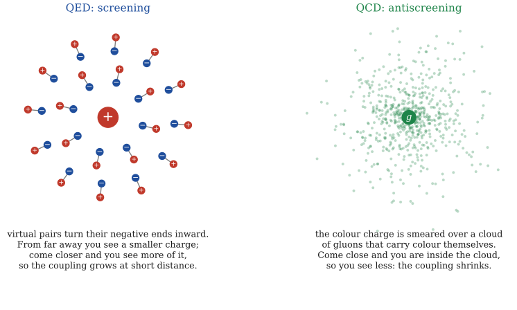
The usual picture. It's a heuristic only; the exact statement is the sign of \(\beta\). QED's vacuum acts like water around an ion and screens a charge. QCD's gluons carry charge themselves and the overall effect is reversed.
The finite part says the same thing. We measure \(\alpha=1/137.036\) with photons of almost zero momentum, so the physical, finite quantity is the change from \(q^2=0\): \(\hat\Pi_2(q^2)=\Pi_2(q^2)-\Pi_2(0)\). The \(2/\epsilon\) is the same at every \(q^2\), so it cancels in the difference. Using step 6 of the recipe in Part 2 for the finite part, what's left is
\[ \hat\Pi_2 = \frac{2\alpha}{\pi}\int_0^1\mathrm d x\,x(1-x)\,\ln\frac{m^2+x(1-x)Q^2}{m^2}, \]where \(Q^2=-q^2>0\) for a spacelike photon. Now take \(Q^2\gg m^2\). Inside the logarithm the \(m^2\) is negligible next to \(x(1-x)Q^2\) (except in tiny corners near \(x=0,1\), which barely contribute), so \(\ln\frac{m^2+x(1-x)Q^2}{m^2}\approx\ln\frac{Q^2}{m^2}+\ln\big(x(1-x)\big)\). Two simple integrals remain:
\[ \int_0^1x(1-x)\,\mathrm d x=\frac16,\qquad \int_0^1x(1-x)\ln\big(x(1-x)\big)\,\mathrm d x=-\frac5{18}. \](For the second, split the log into \(\ln x+\ln(1-x)\). By symmetry the two halves are equal and \(\int_0^1(x-x^2)\ln x\,\mathrm d x=-\tfrac14+\tfrac19=-\tfrac5{36}\).) Putting it together,
\[ \hat\Pi_2(Q^2)\approx\frac{2\alpha}{\pi}\left[\frac16\ln\frac{Q^2}{m^2}-\frac5{18}\right]=\frac{\alpha}{3\pi}\left[\ln\frac{Q^2}{m^2}-\frac53\right],\qquad \alpha_{\rm eff}(Q^2)=\frac{\alpha}{1-\hat\Pi_2(Q^2)}. \]The \(1/(1-\hat\Pi_2)\) is the same geometric series we summed for the propagator in Part 1: a photon can polarise the vacuum once, twice, three times in a row and \(1+\hat\Pi_2+\hat\Pi_2^2+\dots=1/(1-\hat\Pi_2)\).
Differentiate with respect to \(\ln Q\) and you get \(2\alpha^2/3\pi\) back exactly. At \(Q=m_Z\) with only the electron in the loop this gives \(1/\alpha_{\rm eff}=134.65\) (the exact one-loop integral, checked two ways). The measured value is \(1/\alpha(m_Z)=127.95\), because every charged particle lighter than the \(Z\) (the muon, the tau and the quarks) runs in the loop too. The effect is large, it has been measured and the running is exactly as predicted.
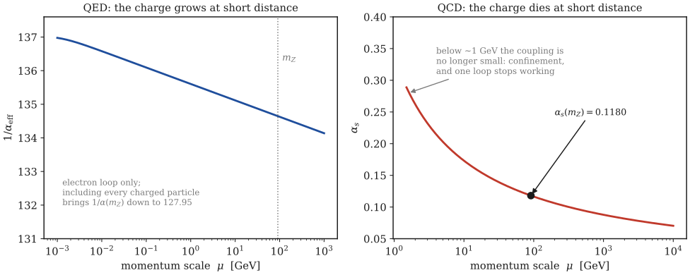
Left: \(1/\alpha\) falls as the energy rises, from the electron loop alone (the exact one-loop integral). Right: the strong coupling \(\alpha_s\) at one loop with five quark types, starting from the measured \(\alpha_s(m_Z)=0.1180\). It falls at high energy.
QCD: asymptotic freedom
The strong force is where running couplings stop being a technical detail. Here the coupling runs the other way from QED, which is the whole reason quarks behave as they do. For 3 colours with \(n_f\) types of quark, the one-loop result is (Gross and Wilczek and Politzer, 1973; worked out in Peskin §16.5 to §16.6):
\[ \beta(g) = -\frac{g^3}{16\pi^2}\left(\frac{11}{3}N-\frac23 n_f\right)\qquad\Longleftrightarrow\qquad \mu\frac{\mathrm d\alpha_s}{\mathrm d\mu}=-\frac{b_0}{2\pi}\alpha_s^2,\quad b_0=11-\frac23n_f\ \ (N=3). \]That line has six symbols in it. None of them is difficult, so here is every one.
Why this one is quoted instead of derived
The QED beta function in the last section came from one diagram, the electron loop, which we traced out in FORM. The QCD one needs three new ingredients that would take a course of their own: gluons carry colour charge so they couple to themselves, which adds diagrams with three and four gluon legs that have no QED counterpart; the gluon propagator needs a gauge choice; and that gauge choice drags in ghosts.
None of that changes the RG logic of this part. The coupling still runs, the beta function is still read off from the \(1/\epsilon\) pole, so Exercise 7.1's formula \(\beta=\rho(ga_1'-a_1)\) still delivers it. Only the diagram count goes up.
Where the sign comes from
You can still see why the answer has the sign it does. The two pieces of \(b_0\) pull in opposite directions.
The quark piece, \(-\tfrac23n_f\), is ordinary screening. A quark loop does exactly what the electron loop did in QED. Virtual quark and antiquark pairs pop out of the vacuum, turn their negative end towards the charge, hiding part of it. Get closer than the cloud and you see more charge. That is why its sign matches QED's.
The gluon piece, \(+\tfrac{11}3N\), is antiscreening. Because a gluon itself carries colour, a colour charge leaks into the cloud around it, so the cloud carries the same colour as the source rather than the opposite one. Peskin §16.7 works this out picture by picture: the induced dipole ends up pointing towards the original charge, amplifying it instead of hiding it. Move away from the source and you see more charge, not less. Move in close and there is less and less of it.
The two effects are inside the same number. Peskin's quantitative statement is that the antiscreening beats the gauge boson screening by a factor of 12, which is exactly what \(\tfrac{11}3=\tfrac{12}3-\tfrac13\) says: a screening piece \(-\tfrac13\) of the ordinary kind, plus an antiscreening piece \(+\tfrac{12}3=4\) that only a self-interacting force can have.
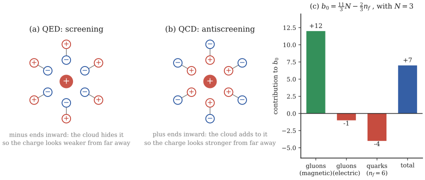
Why QCD runs the other way. (a) In QED the vacuum dipoles turn their minus ends inward, so they hide the charge. (b) In QCD the induced dipole points inward with its plus end, so it adds to the charge. (c) The same story as numbers: the magnetic, self-interaction piece of the gluon gives $+12$, the ordinary screening piece of the gluon gives $-1$, six quark flavours give $-4$. The gluons win, so $b_0>0$ and therefore $\beta<0$.
So \(\tfrac{11}3N\) beats \(\tfrac23n_f\) as long as \(n_f<\tfrac{11}2N=16.5\), which the real world comfortably satisfies with six flavours. Then \(b_0>0\), so \(\beta<0\) and the strong coupling shrinks at high energy. That is asymptotic freedom: quarks squeezed close together stop interacting.
Solving the flow, then reading off \(\Lambda_{\rm QCD}\)
The \(\alpha_s\) equation is easy to integrate. Write it for \(1/\alpha_s\):
\[ \frac{\mathrm d}{\mathrm d\ln\mu}\frac{1}{\alpha_s}=-\frac1{\alpha_s^2}\frac{\mathrm d\alpha_s}{\mathrm d\ln\mu}=\frac{b_0}{2\pi} \qquad\Longrightarrow\qquad \frac{1}{\alpha_s(\mu)}=\frac{1}{\alpha_s(\mu_0)}+\frac{b_0}{2\pi}\ln\frac{\mu}{\mu_0}. \]So \(1/\alpha_s\) climbs as a straight line in \(\ln\mu\). Run the line backwards and it must cross zero somewhere, which means \(\alpha_s\) itself blows up there. Call that place \(\Lambda_{\rm QCD}\) and the solution takes a form with no free constant left in it at all:
\[ \boxed{\;\alpha_s(\mu)=\frac{2\pi}{b_0\,\ln(\mu/\Lambda_{\rm QCD})}\;},\qquad \Lambda_{\rm QCD}=\mu_0\,e^{-2\pi/(b_0\alpha_s(\mu_0))}. \]Putting in \(\alpha_s(m_Z)=0.1180\) with \(n_f=5\) gives \(b_0=23/3\) and \(\Lambda_{\rm QCD}=0.088\) GeV at one loop. The same line then gives \(\alpha_s(1\ \mathrm{TeV})=0.088\) and \(\alpha_s(10\ \mathrm{GeV})=0.173\). Running down to \(2\) GeV gives \(0.262\). Real analyses get about \(0.30\) there, because they use more loops and change \(n_f\) at each quark mass, so treat the one-loop number as a sketch. The blow-up at \(0.09\) GeV signals that the approximation has broken down, not that anything really becomes infinite. It does mark roughly where quarks stop being free objects, which is why the proton's size is what it is.
Run it yourself
Things to try. In QCD, drag \(n_f\) past 16 and watch asymptotic freedom disappear as the curve turns round. In QED with one flavour, find the Landau pole: it's around \(10^{277}\) GeV, absurdly far beyond the Planck scale, so in practice nobody worries about it.
Exercises
Show solution
Show solution
Show solution
Show solution
Show solution
The pole has moved from \(q^2=0\) to \(q^2=M^2\): the photon would have a mass \(M\). Light would then have a finite range, which is ruled out by experiment to an extraordinary precision.
Transverse insertion. Now each insertion brings \(q^2\,\Pi(q^2)\) (the \(q^\mu q^\nu\) part drops out when the photon couples to conserved currents). The chain is
\[ \frac1{q^2}+\frac1{q^2}\,q^2\Pi\,\frac1{q^2}+\dots=\frac1{q^2}\big(1+\Pi+\Pi^2+\dots\big)=\frac{1}{q^2\,\big(1-\Pi(q^2)\big)}. \]The pole stays at \(q^2=0\), so the photon stays massless. What changes is the height of the propagator: every exchange of a photon between two charges is multiplied by \(1/(1-\Pi(q^2))\), which is the same as replacing \(e^2\) by \(e^2/(1-\Pi(q^2))\). That's exactly \(\alpha_{\rm eff}\), the running coupling of this page. (This is Peskin eq. 7.77.)
So the factor of \(q^2\) that the calculation produced, the one that looked like tidy bookkeeping, is precisely what makes the loop change the strength of the force rather than the mass of the photon. And that factor comes from gauge symmetry, which is why the FORM and Wolfram check of transversality in this section matters.