
- From spins to a smooth field
- The field as a sum of waves
- One RG step, in three moves
- The free field: the Gaussian fixed point
- Averaging over the free field, one mode at a time
- What the free field looks like: its correlation function
- Scaling dimensions: power counting is an RG fact
- Why four dimensions is special
- The same answer from fluctuations: the Ginzburg criterion
- Exercises
Renormalisation Group V: Wilson's Momentum Shells
Part 5 of eight. previous: Fixed points and universality · Course home · Glossary · next: The Wilson-Fisher point
Coarse-graining in real space (voting in blocks) gave us the right ideas but rough numbers. Wilson's move was to coarse-grain in momentum space instead. There, "throw away small details" becomes "throw away the fastest wiggles" and perturbation theory gives controlled answers. This part sets up the machinery on a free field, where everything is exact. Part 6 switches on the interaction.
From spins to a smooth field
Block-spin a magnet enough times and each block spin is an average over thousands of original spins. At that point it's better to treat it as a smooth number, the local magnetisation \(\phi(\mathbf x)\), rather than as \(\pm1\).
What's the most general formula for the energy of such a field? Landau and Ginzburg's answer was to write down everything the symmetry allows, as a series in powers of \(\phi\) and its slope and keep the first few terms. The up/down symmetry \(\phi\to-\phi\) rules out odd powers, which leaves
\[ S[\phi] = \int\mathrm d^dx\left[\tfrac12(\nabla\phi)^2 + \tfrac12 r\,\phi^2 + \frac{u}{4!}\phi^4\right], \]where \(r\) is proportional to \(T-T_0\) and changes sign near the transition. The partition function becomes \(Z=\int\mathcal D\phi\,e^{-S[\phi]}\).
This is exactly the Euclidean \(\phi^4\) theory from Part 1, with \(r=m^2\) and \(u=\lambda\). A statistical field theory in \(d\) dimensions and a quantum field theory in \(d\) spacetime dimensions are the same mathematical object, as Part 2 showed with the Wick rotation. That's why a course about magnets is also a course about particles.
The underlying lattice spacing \(a\) means no wave on the field can be shorter than \(a\). In momentum language, the field only has components with \(|\mathbf k|<\Lambda\sim\pi/a\). That's the cutoff and here it's completely physical: it's the size of the atoms.
The field as a sum of waves
Wilson's method works with the waves that make up the field, so let's set that up carefully. Any field can be written as a sum (an integral) of waves, each with a wavevector \(\mathbf k\):
\[ \phi(\mathbf x)=\int\frac{\mathrm d^dk}{(2\pi)^d}\,e^{i\mathbf k\cdot\mathbf x}\,\phi(\mathbf k). \]Since \(\phi(\mathbf x)\) is real, \(\phi(-\mathbf k)=\phi(\mathbf k)^*\). A large \(|\mathbf k|\) is a short, fast wiggle and a small \(|\mathbf k|\) is a long, slow swell. Each wave is called a mode.
Now rewrite the free part of the action in terms of the waves. Take the stiffness term first. Each \(\nabla\) acting on \(e^{i\mathbf k\cdot\mathbf x}\) just brings down \(i\mathbf k\), so
\[ \int\mathrm d^dx\,(\nabla\phi)^2 = \int\frac{\mathrm d^dk}{(2\pi)^d}\frac{\mathrm d^dk'}{(2\pi)^d}\,(i\mathbf k)\cdot(i\mathbf k')\,\phi(\mathbf k)\phi(\mathbf k')\int\mathrm d^dx\,e^{i(\mathbf k+\mathbf k')\cdot\mathbf x}. \]The last integral is the key fact about waves: adding up \(e^{i(\mathbf k+\mathbf k')\cdot\mathbf x}\) over all of space gives zero unless the two waves exactly cancel, \(\mathbf k'=-\mathbf k\). Precisely, \(\int\mathrm d^dx\,e^{i(\mathbf k+\mathbf k')\cdot\mathbf x}=(2\pi)^d\,\delta^d(\mathbf k+\mathbf k')\). The delta function removes the \(\mathbf k'\) integral and sets \(\mathbf k'=-\mathbf k\), so \((i\mathbf k)\cdot(i\mathbf k') = (i\mathbf k)\cdot(-i\mathbf k)=k^2\) and \(\phi(\mathbf k)\phi(-\mathbf k)=|\phi(\mathbf k)|^2\). The mass term works the same way without the \(k\)'s. Together:
\[ S_0=\int\mathrm d^dx\left[\tfrac12(\nabla\phi)^2+\tfrac12r\phi^2\right] = \int\frac{\mathrm d^dk}{(2\pi)^d}\;\tfrac12\,(k^2+r)\,|\phi(\mathbf k)|^2. \]This is a big simplification. In position space, neighbouring points are tied together by the stiffness term. In wave language, every mode is on its own: the action is a separate sum over modes, with no mode talking to any other.
The \(\phi^4\) term is different. Written in waves, it contains four modes at once, \(\phi(\mathbf k_1)\phi(\mathbf k_2)\phi(\mathbf k_3)\phi(\mathbf k_4)\), with the same kind of delta function forcing \(\mathbf k_1+\mathbf k_2+\mathbf k_3+\mathbf k_4=0\). So the interaction lets modes with different wavevectors affect each other, as long as their wavevectors add to zero. That's the only reason coarse-graining is ever hard.
One RG step, in three moves
Split every wave in the field into slow and fast parts:
\[ \phi(\mathbf x) = \phi_{\rm s}(\mathbf x) + \phi_{\rm f}(\mathbf x), \qquad \phi_{\rm s}:\ |\mathbf k|<\Lambda/b,\qquad \phi_{\rm f}:\ \Lambda/b<|\mathbf k|<\Lambda. \]The subscripts are nothing clever: \({\rm s}\) for slow, \({\rm f}\) for fast. (Most books write \(\phi_<\) with \(\phi_>\) instead, meaning below the shell with above it. Same split, harder to read at a glance.) The fast part \(\phi_{\rm f}\) lives in a thin shell in momentum space, just below the cutoff.
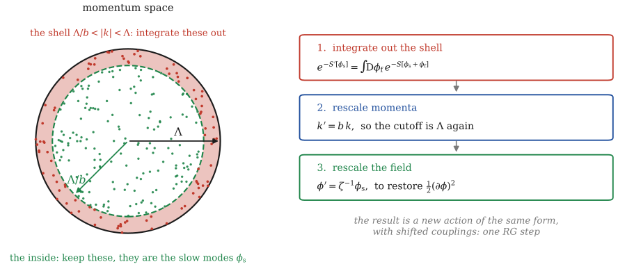
One RG step. Integrate out the fast modes in the shell (red), stretch momenta so the cutoff is back at \(\Lambda\), then rescale the field so its stiffness term looks the same as before. What's left over is a change in the couplings.
Move 1: coarse-grain. Integrate out the shell. That defines a new action for the slow modes alone:
\[ e^{-S'[\phi_{\rm s}]} = \int\mathcal D\phi_{\rm f}\,e^{-S[\phi_{\rm s}+\phi_{\rm f}]}. \]Any question about long-distance physics gets the same answer from \(S'\) as from \(S\). We've changed the description, not the physics.
Move 2: zoom out. The new theory has cutoff \(\Lambda/b\), so it can't be compared directly with the old one. Tong calls them "apples and oranges". So stretch momenta, \(\mathbf k'=b\mathbf k\) (equivalently, shrink lengths, \(\mathbf x'=\mathbf x/b\)), which puts the cutoff back at \(\Lambda\). This is exactly "stepping back from the picture": everything looks smaller.
Move 3: fix the contrast. Rescale the field, \(\phi'=\zeta^{-1}\phi_{\rm s}\), choosing \(\zeta\) so that the stiffness term \(\tfrac12(\nabla\phi)^2\) keeps its standard form. Without this step the stiffness would just drift and we'd never find a fixed point.
After the three moves, the action has the same form with new couplings \((r',u',\dots)\). That's the RG map, now for a field.
The free field: the Gaussian fixed point
Switch the interaction off, \(u=0\). In momentum space the action is then a sum over separate waves that don't talk to each other,
\[ S = \int_{|\mathbf k|<\Lambda}\frac{\mathrm d^dk}{(2\pi)^d}\,\tfrac12(k^2+r)\,|\phi(\mathbf k)|^2, \]Now Moves 2 and 3. Put \(\mathbf k=\mathbf k'/b\), so \(\mathrm d^dk=b^{-d}\mathrm d^dk'\) and \(k^2=b^{-2}k'^2\) and set \(\phi_{\rm s}(\mathbf k'/b)=\zeta\,\phi'(\mathbf k')\):
\[ S' = \int_{|\mathbf k'|<\Lambda}\frac{\mathrm d^dk'}{(2\pi)^d}\,\tfrac12\, b^{-d}\zeta^2\big(b^{-2}k'^2 + r\big)|\phi'(\mathbf k')|^2. \]To keep the coefficient of \(k'^2\) equal to one we need \(\zeta^2=b^{d+2}\) and then
\[ \boxed{\; r' = b^2 r.\;} \]So \(r=0\) is a fixed point: the free, massless field. It's called the Gaussian fixed point, because the weight \(e^{-S}\) is a Gaussian. It has one relevant direction, \(r\), with \(y_r=2\), so \(\nu=1/y_r=\tfrac12\). That's exactly the mean-field value.
Averaging over the free field, one mode at a time
To integrate out the fast modes in Part 6, we'll need averages like \(\langle\phi(\mathbf k)\phi(\mathbf k')\rangle\) over the free weight \(e^{-S_0}\). Since every mode is on its own, each one is just an ordinary Gaussian integral.
Take one variable \(x\) with weight \(e^{-ax^2/2}\). Its normalisation is \(Z(a)=\int\mathrm d x\,e^{-ax^2/2}=\sqrt{2\pi/a}\). Differentiating with respect to \(a\) brings down \(-x^2/2\), so
\[ \langle x^2\rangle = \frac{\int x^2e^{-ax^2/2}\mathrm d x}{\int e^{-ax^2/2}\mathrm d x} = -2\,\frac{\mathrm d\ln Z}{\mathrm d a} = -2\cdot\left(-\frac{1}{2a}\right) = \frac1a. \]For the mode with wavevector \(\mathbf k\), the "\(a\)" is \(k^2+r\). Different modes are independent, so their average is zero unless they're the same mode (really \(\mathbf k\) and \(-\mathbf k\), since \(\phi(-\mathbf k)=\phi(\mathbf k)^*\)):
\[ \boxed{\;\langle\phi(\mathbf k)\phi(\mathbf k')\rangle = (2\pi)^d\,\delta^d(\mathbf k+\mathbf k')\;\frac1{k^2+r}\equiv(2\pi)^d\,\delta^d(\mathbf k+\mathbf k')\,G(k).\;} \]This \(G(k)\) is the propagator from Part 1, now found as a simple average. The delta function says different modes don't know about each other.
Wick's theorem: averages of more fields
Three words are about to be used over and over, so here is what each one means.
What about four fields? For one Gaussian variable, the same differentiation trick gives \(\langle x^4\rangle=3/a^2=3\langle x^2\rangle^2\). The 3 has a simple meaning: it's the number of ways to split four things into two pairs. For many Gaussian variables:
\[ \langle x_1x_2x_3x_4\rangle = \langle x_1x_2\rangle\langle x_3x_4\rangle + \langle x_1x_3\rangle\langle x_2x_4\rangle + \langle x_1x_4\rangle\langle x_2x_3\rangle. \]This is Wick's theorem. The average of any product of Gaussian variables is the sum over all ways of pairing them up, each pair giving a propagator. Averages of an odd number of fields are zero, because there's always one left over with no partner.
Why it's true. The trick is to add a source: an extra term \(Jx\) in the exponent, where \(J\) is just a number we are free to choose. Complete the square, \(-\tfrac a2x^2+Jx=-\tfrac a2\big(x-\tfrac Ja\big)^2+\tfrac{J^2}{2a}\), then shift the integration variable by \(J/a\). The shifted integral is the same one as before, so it cancels against the denominator:
\[ \big\langle e^{Jx}\big\rangle=\frac{\int\mathrm d x\;e^{-ax^2/2+Jx}}{\int\mathrm d x\;e^{-ax^2/2}}=e^{J^2/2a}=e^{J^2\langle x^2\rangle/2}. \]Now expand both sides in powers of \(J\). On the left, \(\sum_n J^n\langle x^n\rangle/n!\). On the right, only even powers survive, since the exponent carries \(J^2\). Matching the coefficient of \(J^{2n}\):
\[ \frac{\langle x^{2n}\rangle}{(2n)!}=\frac1{n!}\left(\frac{\langle x^2\rangle}{2}\right)^{n} \qquad\Longrightarrow\qquad \langle x^{2n}\rangle=\frac{(2n)!}{2^n\,n!}\,\langle x^2\rangle^n=(2n-1)!!\;\langle x^2\rangle^n. \]Two things drop out at once.
Odd averages vanish. The right-hand side has no odd powers of \(J\), so there is nothing for \(\langle x\rangle\), \(\langle x^3\rangle\), \(\langle x^5\rangle\) to match. They are all zero.
The number is the number of pairings. \((2n-1)!!\) means \(1\cdot3\cdot5\cdots(2n-1)\), the double factorial. It counts pairings directly: the first field picks a partner in \(2n-1\) ways, the first of the ones still free picks in \(2n-3\) ways, down to the last pair with one way. Four fields give \(3\), six give \(5\cdot3=15\), eight give \(105\). So the combinatorial factor in the formula is the count of pairings, not a coincidence.
Nothing there used more than one variable. Give each variable its own source and the same completion of the square gives \(\big\langle e^{\sum_iJ_ix_i}\big\rangle=\exp\big(\tfrac12\sum_{i,j}J_iJ_j\langle x_ix_j\rangle\big)\), whose expansion is the sum over pairings with one propagator per pair. That is all we need here, because \(S_0\) is diagonal in momentum: the free field literally is a pile of independent Gaussian variables, one per mode. Wick's theorem for fields is the one-variable result applied mode by mode.
(Checked in Wolfram: \(\langle x^2\rangle=1/a\), \(\langle x^4\rangle=3\langle x^2\rangle^2\), the generating function \(\langle e^{Jx}\rangle=e^{J^2/2a}\), the moments \(\langle x^{2n}\rangle=(2n-1)!!/a^n\) up to \(n=4\) and the vanishing of the odd ones. Tong §3.4 proves the operator form of the same statement, where the fields do not commute. In this course the fields are ordinary numbers inside an integral, so the argument above is the whole proof.)
What the free field looks like: its correlation function
Go back to position space. How strongly is the field at one point related to the field a distance \(R\) away? Transform \(G(k)\) back:
\[ \langle\phi(\mathbf x)\phi(0)\rangle = \int\frac{\mathrm d^dk}{(2\pi)^d}\,\frac{e^{i\mathbf k\cdot\mathbf x}}{k^2+r}. \]In three dimensions, use spherical coordinates with \(\mathbf x\) along the \(z\) axis. The angular integral gives \(\int_{-1}^1 e^{ikR\cos\theta}\,\mathrm d(\cos\theta)=\frac{2\sin kR}{kR}\) and what's left is a standard integral:
\[ \langle\phi(\mathbf x)\phi(0)\rangle = \frac{1}{2\pi^2R}\int_0^\infty\frac{k\sin kR}{k^2+r}\,\mathrm d k = \frac{e^{-R/\xi}}{4\pi R},\qquad \xi=\frac1{\sqrt r}. \](Checked in Wolfram.) Far away, the correlation dies off exponentially over the correlation length \(\xi=r^{-1/2}\). Since \(r\propto T-T_c\), this gives \(\xi\propto|T-T_c|^{-1/2}\), so \(\nu=\tfrac12\), as found above.
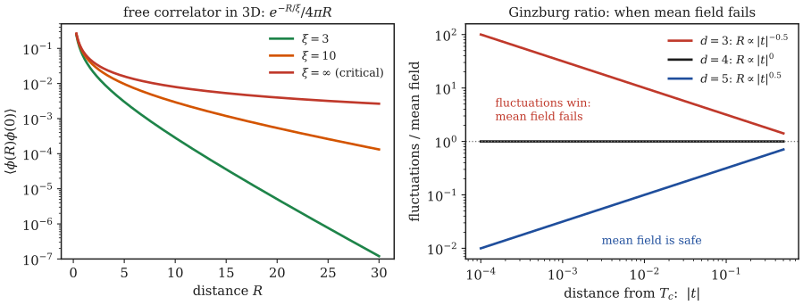
Left: the free correlator in 3D for three correlation lengths. At the critical point it becomes a pure power, \(1/4\pi R\). Right: the Ginzburg ratio, which measures how big fluctuations are compared with the mean-field magnetisation (explained below). Only for \(d>4\) does it stay small near \(T_c\).
At the critical point the correlator is a pure power law, \(1/R^{d-2}\) in \(d\) dimensions. Critical correlations are usually written as \(1/R^{d-2+\eta}\), so the free field has \(\eta=0\). Real 3D magnets have \(\eta=0.036\), which is small but not zero. That tiny difference comes from interactions and it first appears at two loops (Part 6).
Scaling dimensions: power counting is an RG fact
In real space the same rescaling reads \(\mathbf x'=\mathbf x/b\) and \(\phi'(\mathbf x')=b^{(d-2)/2}\phi(\mathbf x)\) (exercise 5.1). The number \((d-2)/2\) is the scaling dimension of \(\phi\) at the Gaussian fixed point. It's the same as the mass dimension \([\phi]\) from Part 1, now showing up as an RG growth rate.
Add any term \(g_n\int\mathrm d^dx\,\phi^n\) and ask how \(g_n\) changes when you zoom out. Since \(\mathrm d^dx=b^d\mathrm d^dx'\) and \(\phi^n=b^{-n(d-2)/2}\phi'^n\),
\[ g_n' = b^{\,y_n}g_n,\qquad y_n = d-n\,\frac{d-2}{2} = [g_n]. \]So near the Gaussian fixed point, how a coupling grows under the RG is just its mass dimension. Positive dimension means relevant, zero means marginal, negative means irrelevant. Terms with derivatives work the same way, with each derivative costing one unit.
The same counting works for a magnetic field, which enters the action as \(-h\int\mathrm d^dx\,\phi\). That's the case \(n=1\): \(y_h=d-\frac{d-2}{2}=\frac{d+2}{2}\). So at the free fixed point the two relevant couplings are temperature, with \(y_t=2\) and field, with \(y_h=\frac{d+2}2\). Put these into the exponent formulas of Part 4 with \(d=4\): \(\nu=\tfrac12\), \(\gamma=\frac{2y_h-d}{y_t}=1\), \(\beta=\frac{d-y_h}{y_t}=\tfrac12\), \(\delta=\frac{y_h}{d-y_h}=3\) and \(\eta=d+2-2y_h=0\). These are exactly the mean-field (Landau) exponents. (Above four dimensions the formulas for \(\beta\) and \(\delta\) need extra care, because the irrelevant \(u\) still controls the size of the magnetisation. This is a subtle point, discussed in Tong §3.3.2.)
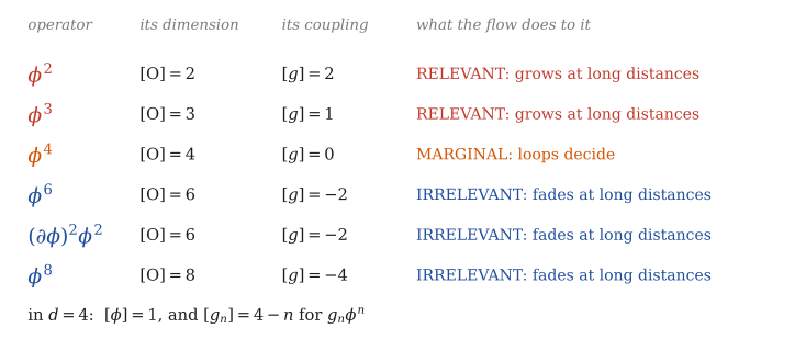
Power counting in four dimensions. The quartic coupling sits right on the boundary (marginal). Anything with more fields or more derivatives is irrelevant.
This is why you only ever write a few terms in a Lagrangian. An irrelevant coupling \(g\) with \([g]=-p\) affects things at energy \(E\) in the combination \(gE^p\), which is suppressed by \((E/\Lambda)^p\) if \(g\sim\Lambda^{-p}\). By the time you coarse-grain down to the scales where you measure things, only the relevant and marginal couplings are left. So the theory you see at low energy is forced to be simple. "Renormalisable" theories, the ones with only non-negative-dimension couplings, aren't a lucky choice by nature. They're what any theory looks like from far enough away. Part 8 comes back to this.
Why four dimensions is special
Apply the formula to the quartic coupling: \(y_4=4-d\).
\(d>4\): \(u\) is irrelevant at the Gaussian point. A critical system flows to the free theory and the mean-field exponents (\(\nu=\tfrac12\) and friends) are exactly right.
\(d=4\): \(u\) is marginal. The simple counting can't decide, so we need loops. Part 6 shows \(u\) is marginally irrelevant: it dies away, but only very slowly, like a logarithm.
\(d<4\): \(u\) is relevant. The Gaussian point now has a second unstable direction, so a critical system can't flow into it. It must flow somewhere else, to a fixed point with \(u^*\neq0\), whose exponents differ from mean field. That's why \(\nu\) for real 3D magnets is \(0.63\), not \(0.5\).
Four is called the upper critical dimension of the Ising class. Wilson and Fisher's idea was to work in \(d=4-\epsilon\) dimensions, where the new fixed point sits at a small coupling \(u^*\) of size \(\epsilon\), so perturbation theory can handle it. That's Part 6.
The same answer from fluctuations: the Ginzburg criterion
There's a second, very physical way to see why four dimensions is special, due to Ginzburg and explained in Tong §2.2.4. Mean-field theory replaces the field by its average value. That's only fair if the fluctuations around the average are small compared with the average itself.
Let's compare the two, below \(T_c\) where \(r<0\).
The average. Minimising the potential \(\tfrac12r\phi^2+\frac{u}{4!}\phi^4\) gives \(r\phi+\frac u6\phi^3=0\), so the mean-field magnetisation is \(m_0^2=\frac{6|r|}{u}\).
The fluctuations. Add up the correlation function over one correlation volume (a ball of radius \(\xi\)). Inside that ball the correlator is roughly \(1/R^{d-2}\) and the ball's shells have area \(\propto R^{d-1}\), so
\[ \int_{|x|<\xi}\mathrm d^dx\,\langle\phi(x)\phi(0)\rangle\sim\int_0^\xi\frac{R^{d-1}}{R^{d-2}}\,\mathrm d R=\int_0^\xi R\,\mathrm d R=\frac{\xi^2}{2}. \]The ratio. Divide by the same volume filled with the mean field, \(\xi^d m_0^2\):
\[ \text{Ratio}\sim\frac{\xi^2}{\xi^dm_0^2}=\frac{\xi^{2-d}}{m_0^2}. \]With \(\xi=|r|^{-1/2}\) and \(m_0^2=6|r|/u\),
\[ \text{Ratio}\sim\frac{|r|^{(d-2)/2}}{6|r|/u}=\frac u6\,|r|^{(d-4)/2}\propto|T-T_c|^{(d-4)/2}. \](Checked in Wolfram.) Near the critical point \(|T-T_c|\to0\), so:
for \(d>4\) the power is positive and the ratio goes to zero: fluctuations become negligible and mean field is exact;
for \(d<4\) the power is negative and the ratio goes to infinity: fluctuations swamp the average and mean field fails;
for \(d=4\) it's borderline and the answer involves logarithms.
Tong's summary is that below four dimensions mean-field theory "predicts its own demise". This is the same \(d=4\) we found from power counting, reached in a completely different way.
Exercises
Show solution
Show solution
Show solution
Show solution
Show solution
Show solution