
Renormalisation Group III: Block Spins
Part 3 of eight. previous: Loops, infinities and cutoffs · Course home · Glossary · next: Fixed points and universality
Part 1 said the numbers in a theory depend on the resolution you describe it at. This part makes that concrete with a system so simple you can coarse-grain it exactly on paper. No field theory is needed at all.
The Ising model
Put a tiny magnet, a spin, on each site of a lattice. Each spin points either up (\(s_i=+1\)) or down (\(s_i=-1\)). Neighbouring spins prefer to point the same way, so the energy is
\[ E = -J\sum_{\langle ij\rangle} s_i s_j , \]summed over neighbouring pairs, with \(J>0\). At temperature \(T\), a configuration appears with probability proportional to \(e^{-E/k_BT}\). Only the combination \(K\equiv J/k_BT\) ever matters, so we call \(K\) the coupling. Large \(K\) means cold, so the spins line up. Small \(K\) means hot, so they point every which way.
Everything we might want to know follows from the partition function, the sum of the weights of all configurations:
\[ Z(K) = \sum_{\{s\}} \exp\Big(K\sum_{\langle ij\rangle}s_is_j\Big). \]If you know QFT, this is a path integral. The "field" is the set of spins, the "action" is \(-K\sum s_is_j\) and summing over all configurations is integrating over all field histories. So coarse-graining this model is the lattice version of integrating out short-distance modes.
Kadanoff's idea: vote in blocks
In 1966 Leo Kadanoff noticed something simple. Near the critical point, spins agree with each other over long distances, so a small block of neighbours mostly points the same way. So replace each block by one "block spin" that points the way the majority of its members point. The result is a lattice with fewer spins and a bigger spacing and it looks like another Ising model, only with a different coupling \(K'\).
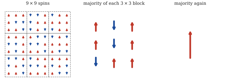
Majority-rule blocking. Each 3×3 block (dashed) is replaced by one spin that points the way most of its members point. Do it again and you have one spin. Each round loses detail. The question is what happens to the coupling between the spins that are left.
Blocking turns the model into itself with a new coupling. That gives a function \(K' = R(K)\), the RG map. Applying it again and again tells us how the system looks from further and further away. In two and three dimensions majority voting can only be done approximately. In one dimension a closely related trick can be done exactly, so that's where we start.
Coarse-graining a line of spins, exactly
Take an endless line of spins with coupling \(K\) between neighbours. Instead of voting, use decimation: sum over every second spin and keep the rest. Look at one removed spin \(s_2\), sitting between two survivors \(s_1\) and \(s_3\). It appears in exactly two bonds, so summing over its two values gives
\[ \sum_{s_2=\pm1} e^{K s_2 (s_1+s_3)} = 2\cosh\big(K(s_1+s_3)\big). \]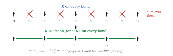
Sum over every even spin. What's left is a line of odd spins, twice as far apart, joined by a new coupling \(K'\).
We want this to look like an ordinary bond between \(s_1\) and \(s_3\), of the form \(f\,e^{K's_1s_3}\), for some new coupling \(K'\) and some constant \(f\). There are only two cases to check:
\[ s_1=s_3:\quad 2\cosh 2K = f\,e^{K'}, \qquad\qquad s_1=-s_3:\quad 2 = f\,e^{-K'}. \]That's two equations for two unknowns. Dividing one by the other gives \(e^{2K'}=\cosh 2K\) and multiplying them gives \(f^2=4\cosh 2K\):
\[ \boxed{\;K' = \tfrac12\ln\cosh 2K \quad\Longleftrightarrow\quad \tanh K' = \tanh^2 K, \qquad f(K) = 2\sqrt{\cosh 2K}.\;} \]The two forms of \(K'\) agree because \(\tanh K' = (e^{2K'}-1)/(e^{2K'}+1) = (\cosh2K-1)/(\cosh2K+1) = \sinh^2K/\cosh^2K\).
What \(\tanh K' = \tanh^2 K\) means
That second form has a lovely meaning. In a line of spins, the number \(\tanh K\) measures how reliably each spin copies its neighbour. (Exactly: the average of \(s_1s_2\) is \(\tanh K\).)
Nothing was approximated here. The partition function of \(N\) spins at coupling \(K\) is a known factor times the partition function of \(N/2\) spins at coupling \(K'\):
\[ Z_N(K) = f(K)^{N/2}\, Z_{N/2}(K'). \]That's one complete, exact RG step. Here's the check in Wolfram Language, which runs as printed:
dec[s1_, s3_] := Exp[K (s1 + s3)] + Exp[-K (s1 + s3)];      (* sum over s2 *)
sol = Solve[{dec[1, 1] == f Exp[Kp], dec[1, -1] == f Exp[-Kp]}, {f, Kp}];
Kp1 = Kp /. First[sol];
FullSimplify[Kp1 - Log[Cosh[2 K]]/2, K > 0]           (* -> 0 *)
FullSimplify[Tanh[Log[Cosh[2 K]]/2] - Tanh[K]^2, K > 0] (* -> 0 *)
FullSimplify[f /. First[sol], K > 0]                   (* -> 2 Sqrt[Cosh[2K]] *)
Following the flow
Now repeat: \(K\to K'\to K''\to\cdots\). Since \(0\le\tanh K<1\), squaring always makes it smaller, so \(K\) goes down at every step. The two ends behave very differently:
Small \(K\) (hot). Use the series \(\tanh K = K-\tfrac13K^3+\dots\), so \(\tanh^2K = K^2-\tfrac23K^4+\dots\). For a small number \(y\), \(\operatorname{artanh}y = y+\tfrac13y^3+\dots\) and \(y^3=K^6\) is far smaller than \(K^4\), so to this order \(K' = \operatorname{artanh}(\tanh^2K) = K^2 - \tfrac23K^4+\dots\). Squaring a small number makes it much smaller, so \(K\) shrinks to zero very fast.
Large \(K\) (cold). Use the other form, \(K'=\tfrac12\ln\cosh2K\). For large \(K\), \(\cosh2K=\tfrac12(e^{2K}+e^{-2K})\approx\tfrac12e^{2K}\), so \(K'\approx\tfrac12\big(2K-\ln2\big)=K-\tfrac12\ln2\). So \(K\) creeps down slowly, by \(\tfrac12\ln2\approx0.347\) per step.
(Both expansions were checked in Wolfram with Series[ArcTanh[Tanh[K]^2], {K, 0, 6}], which gives \(K^2-\tfrac23K^4+\tfrac{32}{45}K^6\).)
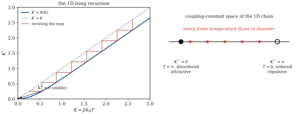
Left: the map \(K'=R(K)\) (blue) lies below the diagonal everywhere, so applying it again and again (red staircase) always walks down to \(K=0\). Right: the same thing drawn as arrows on the line of couplings. There are two fixed points, \(K^*=0\) and \(K^*=\infty\) and every starting point flows to the first one.
The chain's two fixed points are the two ends of the temperature scale. At \(K^*=0\) (infinitely hot), every spin is random, so every scale looks like noise. At \(K^*=\infty\) (absolute zero), every spin agrees, so every scale looks uniform. The flow tells us that any chain at a nonzero temperature, seen from far enough away, looks like the infinitely hot one: disordered.
In the game of telephone, however reliable each person is, a long enough line always scrambles the message. That's the RG's way of saying the one-dimensional Ising model never becomes a magnet, which Ising proved the hard way in 1925.
The correlation length and a small miracle
How far does order reach along the chain? Here's a neat way to find out. Instead of the spins, use the bonds: define \(\tau_i = s_is_{i+1}\), which is \(+1\) if two neighbours agree and \(-1\) if they disagree. The energy is \(-J\sum\tau_i\), so each bond is independent of the others, with probability proportional to \(e^{K\tau_i}\). The average of one bond is therefore
\[ \langle\tau\rangle = \frac{e^{K}\cdot(+1)+e^{-K}\cdot(-1)}{e^{K}+e^{-K}} = \tanh K. \]Now \(s_0s_r = (s_0s_1)(s_1s_2)\cdots(s_{r-1}s_r) = \tau_0\tau_1\cdots\tau_{r-1}\), because each middle spin appears twice and \(s_i^2=1\). Since the bonds are independent, the average of the product is the product of the averages:
\[ \langle s_0s_r\rangle = (\tanh K)^r. \]That's the reliability multiplied \(r\) times, just as in telephone. (Das derives the same result in §15.1 with the transfer matrix, if you'd like a second route.) A power like that decays as \(e^{-r/\xi}\), which defines the correlation length in units of the lattice spacing:
\[ \xi(K) = -\frac{1}{\ln\tanh K}. \]After one decimation the spacing between spins has doubled. A distance that used to be \(2r\) steps is now only \(r\) steps. So if coarse-graining keeps the physics fixed, the correlation length counted in the new steps must be half the old one: \(\xi(K')=\xi(K)/2\). Check it: \(\ln\tanh K' = \ln\tanh^2 K = 2\ln\tanh K\), so \(\xi(K')=\xi(K)/2\)exactly.
This is the most important equation in the course, in its simplest form. Coarse-graining throws away detail but keeps the physics, so after a step of scale factor \(b\):
\[ \xi(K') = \xi(K)/b. \]Now apply it at a fixed point, where \(K'=K\). Then \(\xi=\xi/b\), which only works if \(\xi=0\) or \(\xi=\infty\). A fixed point has either no correlations at all or infinitely long ones. The interesting fixed points, the ones behind phase transitions, are the infinite kind. The chain doesn't have one at any finite \(K\). In two dimensions it does and that's the next part.
Try it
The widget takes a real sample of a chain at coupling \(K\). Each click keeps every second spin. The spins that survive are an exact sample of a chain at the new coupling \(K'\), twice as spread out. The table tracks the coupling and both versions of the correlation length.
Start at \(K=3\) and click a few times. At first \(K\) hardly moves (the slow, large-\(K\) end) and then it drops off a cliff. The last column, the correlation length in the original units, never changes.
Exercises
Show solution
Show solution