
- A map is not wrong for leaving out your street
- The theory we'll use
- How a particle travels: the propagator
- Interactions dress the particle
- Computing the tadpole, step by step
- Stop the integral: the cutoff
- What this is really telling us
- Why plain dimensional analysis isn't enough
- Two roads to the same place
- Exercises
Renormalisation Group I: Why Scale Matters
Part 1 of eight. Course home · Glossary · next: Loops, infinities and cutoffs
A map is not wrong for leaving out your street
It's Durga Puja and you open a map on your phone to go pandal hopping. Zoomed all the way out, West Bengal fills the screen and Kolkata is a single dot. That map isn't wrong. It's just drawn for a scale at which pandals don't exist. Zoom in once and the city splits into neighbourhoods: Bagbazar, Kumartuli, Ballygunge. Zoom in again and your para appears, with the lane that leads to its pandal. One more zoom and you see the gate, the queue and the phuchka stall beside it. Every one of these maps is correct. Each one shows what matters at its own zoom level and leaves out everything smaller.
Physics works this way all the time and we rarely notice because the levels are so far apart. Nobody predicts the flow of water using quarks. We use the Navier-Stokes equation with two numbers, a density and a viscosity, measured in a lab. Those two numbers are all that survives of the molecular chaos once you average over a cubic micron.
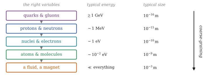
Each rung is a complete theory that works in its own range of sizes. Going down the ladder is coarse-graining: averaging away the small stuff.
David Tong puts it nicely in his lecture notes. Little things affect big things, but they rarely affect very big things. Little things affect slightly bigger things, which affect slightly bigger things again. At each step some information about the start is lost. That is why a biologist studying how starlings flock never needs the Higgs boson.
This sounds like philosophy. It becomes a calculation the moment you work out a quantum correction in field theory, so let's work one out slowly.
The theory we'll use
Take the simplest interacting field theory there is: one real field \(\phi(x)\) that interacts with itself. We work in Euclidean space, which means we have swapped real time \(t\) for imaginary time \(\tau = it\). That one swap turns the oscillating quantum weight \(e^{iS}\) into a real, decaying weight \(e^{-S}\), like a Boltzmann factor, which makes every integral easier. (Part 2 shows why this is allowed.) The action is
\[ S[\phi] = \int \mathrm d^4x \left[ \tfrac12 (\partial\phi)^2 + \tfrac12 m_0^2\phi^2 + \frac{\lambda_0}{4!}\phi^4 \right]. \]The little \(0\) on \(m_0\) and \(\lambda_0\) is a warning. By the end of this page you'll see that these are not the mass and coupling you'd measure in an experiment.
How a particle travels: the propagator
A particle in this theory is a ripple on the sheet. The propagator tells you how easily a ripple with momentum \(p\) travels. Without the interaction it is
\[ G_0(p) = \frac{1}{p^2+m_0^2}. \]The mass hides in this formula. In real (not imaginary) time, the propagator blows up exactly when the particle's energy and momentum satisfy \(E^2 = \mathbf p^2 + m^2\). So the mass is where the propagator has its pole. Keep that in mind, because the interaction is about to move the pole.
Interactions dress the particle
With \(\lambda_0\neq0\), a travelling particle can briefly create a virtual particle and swallow it again. In Feynman-diagram language this is a closed loop attached to the particle's path. The simplest one is called the tadpole, because of its shape.
The real propagator is the sum over every way the particle can travel. It can go straight, or bump once, or bump twice and so on:
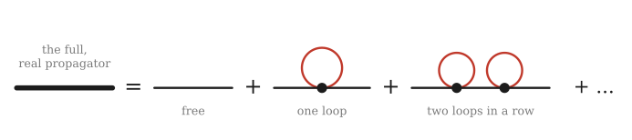
The full propagator (thick line) is the free one, plus the particle bumping once, plus bumping twice in a row and so on forever.
Call the value of one bump (one tadpole, without the two outside lines) \(\Sigma\). Each bump is sandwiched between free propagators and each carries a minus sign (it comes from the \(e^{-S}\) weight), so the series is
\[ G = G_0 - G_0\,\Sigma\,G_0 + G_0\,\Sigma\,G_0\,\Sigma\,G_0 - \dots = G_0\left(1 - \Sigma G_0 + (\Sigma G_0)^2-\dots\right). \]That's a geometric series, \(1-x+x^2-\dots = 1/(1+x)\) with \(x=\Sigma G_0\). Summing it:
\[ G = \frac{G_0}{1+\Sigma G_0} = \frac{1}{G_0^{-1}+\Sigma} = \frac{1}{p^2 + m_0^2 + \Sigma}. \]Look at what happened. The bumps did not change the shape of the propagator; they just added \(\Sigma\) to \(m_0^2\). The pole moved. So the mass you'd measure is
\[ \boxed{\;m^2_{\rm phys} = m_0^2 + \Sigma.\;} \]Everything now depends on computing \(\Sigma\). Let's do it in four steps.
Computing the tadpole, step by step
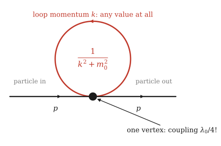
The tadpole with every label. The particle comes in with momentum \(p\) and leaves with \(p\). The loop carries a momentum \(k\) that nothing fixes, so we must add up every value of \(k\).
Step 1: the pieces. A diagram is a product of simple pieces, called the Feynman rules. Take them on trust for now: Part 2 derives every one of them, including the minus sign and the \(\tfrac12\) below, straight from the path integral. The vertex gives the coupling, \(\lambda_0/4!\). The loop is one propagator, \(1/(k^2+m_0^2)\). And since nothing fixes the loop momentum \(k\), we integrate over all of it with \(\int\mathrm d^4k/(2\pi)^4\).
Step 2: the symmetry factor. How many ways can this diagram be made? The vertex \(\phi^4\) has four identical legs. The incoming line can attach to any of the 4 legs and the outgoing line to any of the 3 left. The last two legs then have just one way to join up into the loop. That's \(4\times3 = 12\) ways and dividing by the \(4!=24\) in the coupling leaves \(\tfrac{12}{24}=\tfrac12\).
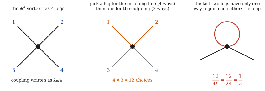
Where the \(\tfrac12\) comes from: 12 ways to attach the two outside lines, divided by the \(4!\) that was put into the coupling.
Putting steps 1 and 2 together:
\[ \Sigma = \frac{\lambda_0}{2}\int\frac{\mathrm d^4k}{(2\pi)^4}\,\frac{1}{k^2+m_0^2}. \]Step 3: use four-dimensional spherical coordinates. The integrand only depends on the length \(k=|k|\), so we can use shells, the same way you'd do a 3D integral with \(\mathrm d^3k = 4\pi k^2\,\mathrm d k\). In four dimensions the "area" of a shell of radius \(k\) is \(2\pi^2k^3\), so \(\mathrm d^4k = 2\pi^2k^3\,\mathrm d k\). The constants combine as \(\frac{\lambda_0}{2}\cdot\frac{2\pi^2}{(2\pi)^4} = \frac{\lambda_0}{16\pi^2}\), leaving one ordinary integral:
\[ \Sigma = \frac{\lambda_0}{16\pi^2}\int_0^{\infty}\frac{k^3\,\mathrm d k}{k^2+m_0^2}. \]Step 4: look at large \(k\). When \(k\) is much bigger than \(m_0\), the integrand is about \(k^3/k^2 = k\). And \(\int^\infty k\,\mathrm d k\) is infinite. It grows like the square of the upper limit.
So the theory, taken at face value, predicts that the particle's measured mass is infinite. That's obviously wrong: particles have finite masses. Something in our reasoning has to give.
Stop the integral: the cutoff
Which part of the integral caused the trouble? Very large \(k\). A loop momentum \(k\) describes a fluctuation of size about \(1/k\), so very large \(k\) means fluctuations at extremely short distances. We integrated all the way to \(k=\infty\), which means we assumed our simple theory is correct down to zero distance.
We have no right to assume that. We haven't tested nature at arbitrarily short distances. So let's be honest and stop the integral at some large momentum \(\Lambda\), called the cutoff:
With the cutoff, the integral is finite. Write \(\frac{k^3}{k^2+m^2} = k - \frac{m^2k}{k^2+m^2}\) and integrate each piece:
\[ \int_0^\Lambda \frac{k^3\,\mathrm d k}{k^2+m_0^2} = \frac12\left[\Lambda^2 - m_0^2\ln\!\Big(1+\frac{\Lambda^2}{m_0^2}\Big)\right], \]and so
\[ \boxed{\;\Sigma = \frac{\lambda_0}{32\pi^2}\left[\Lambda^2 - m_0^2\ln\!\Big(1+\frac{\Lambda^2}{m_0^2}\Big)\right].\;} \]Here's the check in Wolfram Language:
Integrate[k^3/(k^2 + m^2), {k, 0, L}, Assumptions -> {m > 0, L > 0}]
(* (L^2 - m^2 Log[1 + L^2/m^2])/2 *)
(lam/2) (2 Pi^2/(2 Pi)^4) %  // Simplify
(* lam (L^2 - m^2 Log[1 + L^2/m^2])/(32 Pi^2) *)
The measured mass is now finite, \(m^2_{\rm phys}=m_0^2+\Sigma\). But it depends on \(\Lambda\), a number we chose ourselves. If you pick a bigger pixel size, you get a different answer. That looks like a disaster.
What this is really telling us
There are two ways to react.
The old way says: \(\Lambda\) is a trick, so choose \(m_0^2\) to cancel the \(\Lambda^2\) and let \(\Lambda\to\infty\) at the end. That works (Part 7 shows exactly how), but it feels like cheating.
The modern way, due mostly to Kenneth Wilson around 1971, says this is not a disaster at all. It is the most important fact in the story. The Lagrangian is a map drawn at resolution \(\Lambda\). Its numbers \(m_0\) and \(\lambda_0\) aren't "the" mass and "the" coupling. They're the right numbers for a description in which everything smaller than \(1/\Lambda\) has already been averaged away. If you redraw the map at a different resolution, you need different numbers, chosen so that everything you can measure stays the same.
So the sentence "the fine-structure constant is \(1/137\)" is incomplete. It's \(1/137.036\) when you probe an electron very gently. At the energy of the \(Z\) boson it's about \(1/128\). This is a measured fact and Part 7 explains it.
Why plain dimensional analysis isn't enough
One more idea before we set off. With \(\hbar=c=1\), every quantity has a dimension that is some power of mass. The action has none and \(\mathrm d^4x\) has mass dimension \(-4\), so the Lagrangian has dimension \(4\). From the stiffness term \((\partial\phi)^2\) we get \([\phi]=1\) and then \([\lambda_0\phi^4]=4\) forces \([\lambda_0]=0\). In four dimensions the coupling is a pure number.
Here's the puzzle. If \(\lambda\) is a pure number and there's no other scale around (say \(m=0\)), dimensional analysis says a scattering rate can't depend on the collision energy at all. Yet a one-loop calculation gives terms like \(\ln(E/\Lambda)\). The cutoff, the scale we "didn't care about", sneaks back in through a logarithm.
Two roads to the same place
The RG was discovered twice.
On the statistical physics road (Kadanoff 1966, Wilson 1971), people asked why systems as different as a magnet and a boiling liquid behave identically near their critical points. The answer came from literally coarse-graining a lattice. We take this road first, in Parts 3 to 6, because every step can be seen.
On the particle physics road, people asked how the parameters of a quantum field theory depend on the energy at which you measure them. Dmitry Shirkov tells this story in the CERN Courier article "Fifty years of the renormalization group". Stueckelberg and Petermann saw first, in 1951 and 1953, that the rescalings form a group, but their short note "remained unnoticed" and the longer paper was in French. Gell-Mann and Low found the energy dependence of the electric charge in 1954. Bogoliubov and Shirkov then tied these together into a practical algorithm, the "renormalization group method", in 1955 and 1956 and Callan and Symanzik wrote down its modern equation in 1970. That's Part 7.
They turn out to be the same idea. The best moment in the course comes in Part 7, when a number we find by coarse-graining in Part 6 comes back, to the digit, from a completely different calculation.
Exercises
Show solution
Show solution
Show solution