
The Expanding Universe IV — Our Universe
Part 4 of five. Three posts of machinery — geometry, kinematics, dynamics — so we can plug in the numbers of the universe we actually live in, and check the code reproduces them. One post to go: how this smooth background grows the structure we see.
Our universe is "simple but strange": a handful of parameters fix everything in this course, yet we understand almost none of them from first principles. Here we list them, feed them to Cosmic.jl, and compare against Baumann's Table 2.1.
The cosmic inventory — deriving the photon density
Start with the best-measured quantity in cosmology, the CMB temperature \(T_0=2.7260\,\mathrm K\). A blackbody at temperature \(T\) has photon number and energy densities
\[ n_\gamma = \frac{2\zeta(3)}{\pi^2}\left(\frac{k_{\rm B} T}{\hbar c}\right)^3 \approx 410\,\mathrm{cm^{-3}}, \qquad \rho_\gamma c^2 = \frac{\pi^2}{15}\frac{(k_{\rm B} T)^4}{(\hbar c)^3} \approx 4.6\times10^{-34}\,\mathrm{g\,cm^{-3}}\cdot c^2 . \]Dividing \(\rho_\gamma\) by the critical density \(\rho_{c,0}=3H_0^2/8\pi G\) from Part 3 gives the photon density parameter \(\Omega_\gamma\approx5.4\times10^{-5}\). Adding the relic neutrinos (relativistic, \(\Omega_\nu\approx0.68\,\Omega_\gamma\) when massless) gives a total radiation density \(\Omega_r\approx9\times10^{-5}\) — negligible today, but dominant early on because it scales as \(a^{-4}\). The rest is matter (\(\Omega_m\approx0.31\)) and dark energy (\(\Omega_\Lambda\approx0.69\)), with curvature consistent with zero.
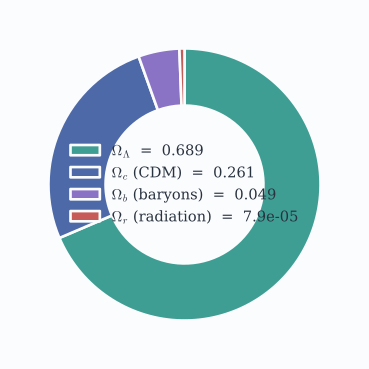
The present-day energy budget, straight from cosmology(). Dark energy dominates, cold dark matter is the bulk of the matter, baryons — everything we are made of — are a few percent, and radiation is a sliver. We understand the physics of only that thin baryonic slice.
Cosmic.jl versus Baumann's Table 2.1
The headline check of the series. The default cosmology() is Planck 2018 ΛCDM; each number is one call, set beside Baumann's value.
| Quantity | Cosmic.jl | Baumann Table 2.1 | call |
|---|---|---|---|
| \(H_0\) [km/s/Mpc] | \(67.66\) | \(67.74 \pm 0.46\) | 100c.h |
| \(\Omega_b\) | \(0.0490\) | \(0.0486 \pm 0.0010\) | Ω_b(c) |
| \(\Omega_m\) | \(0.310\) | \(0.3089 \pm 0.0010\) | Ω_m(c) |
| \(\Omega_\Lambda\) | \(0.689\) | \(0.6911 \pm 0.0062\) | Ω_de(c) |
| \(\Omega_\gamma\) | \(5.40\times10^{-5}\) | \(5.35\times10^{-5}\) | Ω_γ(c) |
| \(\Omega_r\) | \(7.9\times10^{-5}\) | \(8.99\times10^{-5}\) | Ω_r(c) |
| age \(t_0\) [Gyr] | \(13.79\) | \(13.799 \pm 0.021\) | age(c) |
| \(z_{\rm eq}\) | \(3388\) | \(3395 \pm 33\) | z_equality(c) |
Most rows agree to a fraction of a percent — the tiny offsets are Cosmic's Planck-2018 parameters versus the slightly older values Baumann tabulated. Every entry is the code integrating the Friedmann equation from Part 3.
The one row that genuinely differs is instructive: Cosmic's \(\Omega_r=7.9\times10^{-5}\) counts only what is relativistic today — photons and the two massless neutrino species — whereas Baumann's \(8.99\times10^{-5}\) assumes all three neutrinos relativistic. Cosmic knows the third neutrino has mass (\(0.06\,\mathrm{eV}\) by default) and has turned non-relativistic, so it books that species as matter in \(\Omega_\nu\approx1.4\times10^{-3}\). It is the same physics that made the naive \(\rho_r/\rho_m\) crossing in Part 3 disagree slightly with the true \(z_{\rm eq}\): massive neutrinos refuse to be pure radiation or pure matter, and a per-species code gets it right.
So which number is physically right? Cosmic's. A species is relativistic when its thermal momentum exceeds its rest mass, \(k_{\rm B} T_\nu\gg m_\nu c^2\). The relic neutrino background today has \(k_{\rm B} T_\nu\approx1.68\times10^{-4}\,\mathrm{eV}\) — four orders of magnitude below \(m_\nu=0.06\,\mathrm{eV}\) — so that neutrino's typical speed today is \(v/c\sim T_\nu/m_\nu\sim3\times10^{-3}\): it is thoroughly non-relativistic, diluting as \(a^{-3}\) like any other matter, not \(a^{-4}\). Booking it under \(\Omega_r\) at \(z=0\), as Baumann's Table 2.1 number implicitly does, over-counts today's radiation. Baumann's convention is not wrong so much as it is answering a different, and narrower, question: "\(\Omega_r\)" there is really shorthand for the standard \(N_{\rm eff}=3.046\) formula used to fix \(z_{\rm eq}\), and it is an excellent approximation for exactly that purpose — at \(z_{\rm eq}\sim3400\), \(k_{\rm B} T_\nu(z_{\rm eq})\sim0.6\,\mathrm{eV}\gg0.06\,\mathrm{eV}\), so even the massive species is still ultra-relativistic back then and the two conventions agree to high precision (compare z_equality(c) above: \(3388\) versus Baumann's \(3395\), well within their errors). The conventions only diverge once you ask what is relativistic today, and there Cosmic's species-by-species bookkeeping is the one actually tracking the physics.
julia> using Cosmic

julia> c = cosmology();

julia> 100*c.h                   # the Hubble constant H₀, in km/s/Mpc
67.66

julia> Ω_m(c), Ω_de(c)           # matter and dark-energy fractions today
(0.30967, 0.68884)

julia> age(c)                    # the age of the universe, in Gyr
13.787

julia> z_equality(c)             # redshift of matter–radiation equality
3388.0
Matter–radiation equality. Since \(\rho_r/\rho_m\propto a^{-1}\), radiation and matter were equal at \(a_{\rm eq}=\Omega_r/\Omega_m\), i.e. \(z_{\rm eq}\approx3400\), about \(50\,000\) years after the Bang. Everything before was radiation-dominated (\(a\propto t^{1/2}\)); everything after, until dark energy, matter-dominated (\(a\propto t^{2/3}\)). That crossover organises the whole thermal history.
julia> age(c, z_equality(c)) * 1e9    # cosmic time at equality, in years
51400.0
Deriving the thermal history: recombination
The universe was not only denser in the past but hotter: \(T\propto a^{-1}\), so run backwards it is a furnace. At \(z\gtrsim1100\) it was hot enough to keep hydrogen ionised — a plasma of free electrons and protons, opaque because photons Thomson-scatter off the free electrons. As it cooled below \(\sim3000\,\mathrm K\), electrons and protons combined into neutral hydrogen — recombination — the free electrons disappeared, and the universe became transparent. That released light is the CMB.
The Saha equation. In chemical equilibrium the reaction \(e^-+p\leftrightarrow \mathrm H+\gamma\) balances, and the number densities obey the Saha relation. Writing the free-electron fraction \(x_e\equiv n_e/n_b\) (with \(n_b\) the baryon density and, for hydrogen, \(n_e=n_p\)),
\[ \frac{x_e^2}{1-x_e} = \frac{1}{n_b}\left(\frac{m_ek_{\rm B} T}{2\pi\hbar^2}\right)^{3/2} e^{-B_{\rm H}/k_{\rm B} T} ,\]where \(B_{\rm H}=13.6\,\mathrm{eV}\) is the hydrogen binding energy. The exponential is the key: recombination waits until \(k_{\rm B} T\) has fallen well below \(B_{\rm H}\), because the enormous photon-to-baryon ratio (\(n_\gamma/n_b\sim10^9\)) means even the rare high-energy photons in the tail can re-ionise a neutral atom. So recombination happens not at \(T\sim B_{\rm H}/k_{\rm B}\sim1.6\times10^5\,\mathrm K\) but at \(T\sim3000\,\mathrm K\), i.e. \(z\sim1100\). Saha gets where recombination starts right — but it silently assumes the reaction is fast enough to stay in equilibrium at every instant, and that assumption is about to fail.
Why Saha breaks, and the Peebles equation that replaces it. Chemical equilibrium holds only while the recombination rate beats the expansion rate, \(n_b\alpha\gg H\). As \(x_e\) falls, so does the rate of recombination (it needs a free electron to bump into a proton), while \(H\) barely changes — so the reaction inevitably loses the race. Below \(z\sim1600\) or so, electrons and protons are combining slower than equilibrium would predict, and the true \(x_e(z)\) freezes out above the Saha curve: recombination is less complete, and takes longer, than the equilibrium answer suggests. Below that redshift you need the actual rate (Boltzmann) equation for \(x_e\), not the equilibrium condition.
There's a second subtlety hiding in "recombination happens." An electron capturing directly onto the \(n=1\) ground state emits a \(13.6\,\mathrm{eV}\) photon that instantly photoionises the next atom over — net effect: nothing. This is why recombination coefficients are quoted as Case B, \(\alpha_B(T)\): captures to the ground state are excluded from the start, because they don't count. Net recombination has to go through an excited state and then leak to the ground state by a channel the plasma can't immediately undo — either a Lyman-\(\alpha\) photon that redshifts out of resonance before it finds another atom, or the far slower two-photon \(2s\to1s\) decay (splitting the \(10.2\,\mathrm{eV}\) across two photons means neither one alone can re-excite the next atom). Balancing captures into the excited states against these two escape channels, weighted by the Peebles "C factor" for how much of each recombination event actually escapes, gives the (hydrogen-only, effective 3-level) rate equation
\[ \frac{\mathrm d x_e}{\mathrm d t} = -\,C(z)\Big[\underbrace{n_b\,\alpha_B(T)\,x_e^2}_{\text{recombinations}} \;-\; \underbrace{\beta(T)\,(1-x_e)\,e^{-E_{2s1s}/k_{\rm B} T}}_{\text{photoionisations of }n=2}\Big], \qquad C = \frac{\Lambda_{2s1s}+\Lambda_{\alpha}}{\Lambda_{2s1s}+\Lambda_\alpha+\beta} ,\]where \(\beta\) is the photoionisation rate out of \(n=2\) (related to \(\alpha_B\) by detailed balance), \(\Lambda_{2s1s}\approx8.22\,\mathrm{s^{-1}}\) is the two-photon rate, and \(\Lambda_\alpha\) is the cosmological Lyman-\(\alpha\) escape rate — a redshifting-photon effect that only exists because the universe is expanding, with no flat-spacetime analogue. \(C\) is the bottleneck made explicit: it is the fraction of captures into \(n=2\) that actually reach the ground state before being undone, and it is small precisely when \(\beta\) (re-ionisation back out of \(n=2\)) is fast. This is what turns recombination from an instantaneous equilibrium into a genuine rate-limited process, and it's why the true ionisation history trails behind the naive Saha curve.
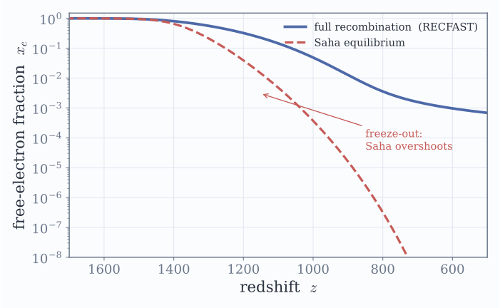
The naive equilibrium answer (Saha, dashed) against the true rate-limited history (solid), both from Cosmic.jl on the same species list. Saha recombines too fast and too completely: once \(x_e\) drops enough that captures can't keep pace with the Hubble expansion, the real universe is left more ionised than equilibrium predicts, at any given redshift — the freeze-out the Peebles \(C\) factor describes.
Cosmic doesn't stop at the textbook two-level Peebles treatment above — it implements the full RECFAST 1.5 system (Wong, Moss & Scott 2008), an effective three-level atom for both hydrogen and helium with a separately-evolved matter temperature, plus a set of correction terms (a retuned fudge factor, a Lyman-\(\alpha\) escape correction, Sobolev escape and H I continuum opacity for helium, the forbidden \(2^3P_1\to1^1S_0\) helium line) that are fitted against genuine multi-level-atom codes — HyRec and CosmoRec, which solve \(\sim100\) atomic shells directly. Is this what CLASS does? Essentially yes: CLASS's default thermodynamics module is its own RECFAST-family implementation at the same level of approximation (\(\sim0.1\%\) on \(x_e\)), and, like Cosmic, it can optionally hand the hydrogen recombination off to a tabulated HyRec model for the last digit of precision — Cosmic exposes exactly that switch as hydrogen = :recfast (default) or :hyrec. What Cosmic does not reimplement is a genuine \(\sim100\)-shell multi-level solve from scratch; it uses the same shortcut every Boltzmann code in production use makes, because the correction terms already absorb the multi-level physics to well beyond the precision this course needs.
julia> saha_x_e(c, 1200.0)         # equilibrium: assumes instant recombination
0.0391

julia> x_e(r, 1200.0)              # the real, rate-limited history
0.3218
At \(z=1200\) equilibrium says recombination is essentially over (\(x_e\approx4\%\)); the real universe is still eight times more ionised than that. The gap only widens going forward — by \(z=1000\) it's a factor of \(130\) — because Saha's exponential is far steeper than the true freeze-out curve once the reaction can no longer keep pace with \(H\). The Peebles \(C\) factor is exactly what is missing from the equilibrium picture.
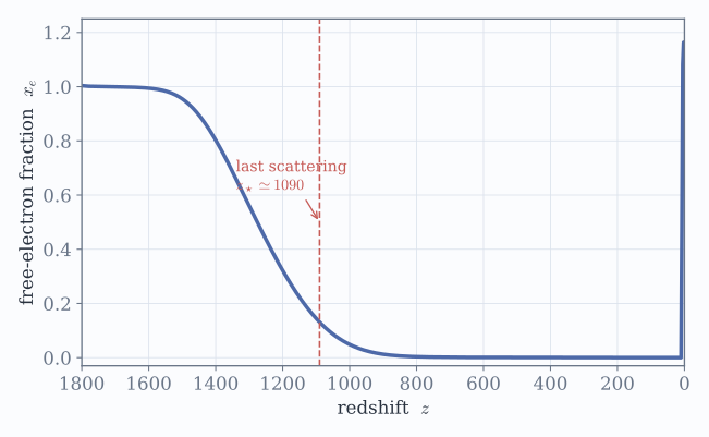
The free-electron fraction \(x_e(z)\) from recombination(c). Reading right to left (forward in time): fully ionised (\(x_e=1\)) until \(z\sim1300\), then a plunge as electrons bind into neutral hydrogen. The dashed line is the surface of last scattering \(z_\star\), where the CMB decoupled. (The small rise back toward \(x_e\approx1.16\) at \(z\to0\) is late reionisation by the first stars, with the extra electrons from ionised helium.)
Two numbers fall out of this calculation, and they anchor precision cosmology. Let me say plainly what each one is:
Cosmic computes the whole thermal history from the species list:
julia> r = recombination(c);

julia> x_e(r, 1400.0)            # free-electron fraction — still mostly ionised
0.803

julia> x_e(r, 1100.0)            # nearly neutral now
0.145

julia> z_star(r)                 # redshift of last scattering (the CMB's "surface")
1089.8

julia> sound_horizon(c, z_star(r))    # comoving sound horizon at last scattering, in Mpc
144.57

julia> r_drag(r)                 # the BAO standard ruler, in Mpc
147.23
That \(147\,\mathrm{Mpc}\), computed on a laptop from a species list, is the same ruler the Planck and DESI collaborations use to map the expansion of the universe — a satisfying place for a background-cosmology package to land.
The end of the beginning
Four posts ago we had two words, homogeneous and isotropic. From them we derived the Robertson–Walker geometry, the redshift and distances, the Friedmann equations and their solutions, and arrived at a quantitative universe that a small Julia package reproduces to the percent level. That is the homogeneous universe, complete.
But perfectly homogeneous is exactly what the real universe isn't — and a good thing too, or there would be no galaxies, no stars, no us. The CMB itself carries \(\Delta T/T\sim10^{-5}\) ripples on top of the smooth background we've been computing. Part 5 — Perturbations picks up exactly there: how those tiny ripples grow under gravity, on the same expanding background this post just pinned down, into the structure we actually observe.
← Back to the course overview.