
The Expanding Universe V — Perturbations
Part 5 of five. The first four posts built a perfectly smooth universe — one function (a(t)), the same everywhere. This post breaks that symmetry on purpose: we perturb the smooth background and derive how the tiny ripples left over from the early universe grow, under their own gravity, into galaxies, clusters, and the pattern of hot and cold spots in the CMB.
Everything so far has been the background: a homogeneous, isotropic universe with one degree of freedom, \(a(t)\). It is a good approximation — the CMB is uniform to 1 part in \(10^5\) — but it is only an approximation, and the \(10^{-5}\) is the most important number in structure formation. Without it, gravity would have nothing to amplify, and the universe today would still be a uniform gas. We now derive how that works: first the Newtonian version, which is intuitive and gets the late-time physics right, then the full relativistic treatment, which is required on large scales and during the radiation era, and which is what Cosmic.jl actually solves.
Newtonian structure formation
Deriving the fluid equations
Treat matter as a pressureless fluid living on the expanding background. Split physical position into a comoving coordinate times the scale factor, \(\vec r = a(t)\vec x\), and split the velocity into the Hubble flow plus a peculiar velocity \(\vec u\equiv a\dot{\vec x}\) — the part left over after subtracting the uniform expansion. Density is \(\rho(\vec x,t)=\bar\rho(t)\big(1+\delta(\vec x,t)\big)\), defining the density contrast \(\delta\equiv\delta\rho/\bar\rho\).
Mass conservation, momentum conservation (sourced by a Newtonian potential \(\Phi\)), and the Poisson equation, written in comoving coordinates and linearised in the small quantities \(\delta,\vec u\):
\[ \dot\delta + \frac1a\nabla\!\cdot\!\vec u = 0 \qquad\text{(continuity)}, \qquad \dot{\vec u} + H\vec u = -\frac1a\nabla\Phi \qquad\text{(Euler)}, \qquad \nabla^2\Phi = 4\pi Ga^2\bar\rho\,\delta \qquad\text{(Poisson)}.\]The Hubble friction term \(H\vec u\) in Euler's equation is new — it is expansion dragging down peculiar velocities, and it is the whole reason structure grows as a power law in an expanding universe rather than exponentially, as it would in static space. Differentiate the continuity equation once more and substitute the other two to eliminate \(\vec u\) and \(\Phi\) (the algebra is two lines: take \(\partial_t\) of continuity, insert \(\dot{\vec u}\) from Euler, then use continuity again to trade \(\nabla\!\cdot\!\vec u\) for \(-\dot\delta\), and Poisson to trade \(\nabla^2\Phi\) for \(\delta\)):
\[ \boxed{\;\ddot\delta + 2H\dot\delta - 4\pi G\bar\rho\,\delta = 0\;} \]No spatial derivatives survive — every Fourier mode \(\delta_k(t)\) obeys the same ODE, independent of \(k\). That is a special feature of pressureless matter (no sound speed to introduce a scale) and it will not survive once we add radiation.
The growing and decaying modes
In matter domination, \(a\propto t^{2/3}\), so \(H=\tfrac23 t^{-1}\) and, from the background Friedmann equation with \(\Omega_m=1\), \(4\pi G\bar\rho=\tfrac32H^2=\tfrac23t^{-2}\). Try a power law \(\delta\propto t^n\):
\[ n(n-1) + \tfrac43n - \tfrac23 = 0 \;\Longrightarrow\; 3n^2+n-2=0 \;\Longrightarrow\; n=\tfrac23 \ \text{or}\ n=-1 .\] \[ \delta_+(t)\propto t^{2/3}\propto a \qquad\text{(growing mode)}, \qquad \delta_-(t)\propto t^{-1}\propto a^{-3/2} \qquad\text{(decaying mode)}.\]Any initial perturbation is a mix of the two, but the decaying mode is irrelevant after a few expansion times — the growth factor \(D(a)\), normalised to \(D(1)=1\) today, tracks the surviving growing mode, and in matter domination \(D(a)=a\) exactly.
From Newtonian to relativistic
The Newtonian equations above are correct once a mode is well inside the horizon and matter dominates the energy budget. They say nothing about scales outside the horizon (where "peculiar velocity" isn't even well defined relative to a fixed background) or about the radiation era, where the dominant species has pressure and free-streams. For that we need the metric itself to fluctuate.
The perturbed metric, and what "gauge" means
Perturb the Robertson–Walker metric of Part 1 with two scalar potentials, in what's called the conformal Newtonian (longitudinal) gauge:
\[ \mathrm d s^2 = a^2(\tau)\Big[-(1+2\Psi)\,\mathrm d\tau^2 + (1-2\Phi)\,\delta_{ij}\,\mathrm d x^i\mathrm d x^j\Big] . \]\(\Psi\) is the direct relativistic generalisation of the Newtonian potential from the section above; \(\Phi\) perturbs the spatial curvature of each constant-\(\tau\) slice. Writing the metric this way already made a choice: General Relativity doesn't come with a preferred coordinate system, so "the density perturbation at this point" is ambiguous until you say which points in the perturbed spacetime correspond to which points of the unperturbed background — that choice is a gauge. A different, equally valid choice (the same physical spacetime, different coordinates) gives a different-looking \(\delta(\vec x,\tau)\), even though nothing physical has changed. This is not a philosophical nicety: superhorizon "perturbations" can look wildly different, or even vanish, in a badly chosen gauge, and getting this wrong is a classic way to derive nonsense.
The Newtonian gauge above is a convenient choice — it fixes the coordinates completely (no leftover freedom) and \(\Psi,\Phi\) reduce directly to Newtonian intuition on subhorizon scales — but it isn't the only one, and it isn't even what the fastest numerical codes traditionally use internally (CAMB and CLASS integrate in the synchronous gauge instead, for numerical-stability reasons, then convert). Cosmic.jl solves and stores everything in the Newtonian gauge and provides gauge_shift to translate a solution into synchronous, comoving, uniform-density or spatially-flat gauge on demand — plus the gauge-invariant combinations, curvature_ℛ and curvature_ζ, and the Bardeen potentials, which take the same value in every gauge and are what you want whenever two different codes need to agree on something physical.
The relativistic fluid equations
Perturbing the stress-energy tensor of a fluid with equation of state \(w\) and sound speed \(c_s^2\), and the Einstein equations that source \(\Phi,\Psi\) from it, gives (in Fourier space, with \(\theta\) the divergence of the peculiar velocity and \(\sigma\) the anisotropic stress):
\[ \dot\delta = -(1+w)(\theta-3\dot\Phi) - 3\mathcal H(c_s^2-w)\delta, \qquad \dot\theta = -\mathcal H(1-3w)\theta + \frac{c_s^2}{1+w}k^2\delta - k^2\sigma + k^2\Psi ,\] \[ k^2\Phi + 3\mathcal H(\dot\Phi+\mathcal H\Psi) = -4\pi Ga^2\,\delta\rho_{\rm com} , \qquad k^2(\Phi-\Psi) = 12\pi Ga^2(\bar\rho+\bar P)\sigma .\]The first pair is the relativistic continuity and Euler equations — one per species — valid for any fluid with constant \(w\) (matter, radiation, a bare \(\Lambda\)); a time-varying equation of state adds one more term, \(-\dot w/(1+w)\,\theta\), to the second equation, which Cosmic.jl carries for quintessence-like dark energy but which vanishes for every species this post actually uses. Cosmic.jl integrates exactly this system (plus the full Boltzmann hierarchy for photons and neutrinos, which don't behave as simple fluids once they start free-streaming). The second pair is the relativistic Poisson equation and the anisotropic-stress equation: \(\sigma\) is sourced only by free-streaming radiation, so in a universe with just matter and \(\Lambda\), \(\Phi=\Psi\) exactly — the two potentials only split apart while photons and neutrinos are around.
Consistency check: recovering Newton. For pressureless matter (\(w=c_s^2=\sigma=0\)) deep inside the horizon, where \(\dot\Phi\) is negligible next to \(\theta\), this collapses to \(\dot\delta_m=-\theta_m\), \(\dot\theta_m=-\mathcal H\theta_m+k^2\Psi\). Combine them, use \(\Phi=\Psi\) and the subhorizon Poisson equation \(k^2\Psi\approx-4\pi Ga^2\bar\rho_m\delta_m\), and convert conformal-time derivatives to cosmic time (\(\mathrm d/\mathrm d\tau=a\,\mathrm d/\mathrm d t\)):
\[ \ddot\delta_m^{(\tau)} + \mathcal H\dot\delta_m^{(\tau)} + k^2\Psi = 0 \;\xrightarrow{\ \tau\to t\ }\; \ddot\delta_m + 2H\dot\delta_m - 4\pi G\bar\rho_m\delta_m = 0 , \]exactly the Newtonian equation derived above. The relativistic machinery isn't a different theory of structure growth — it's the same physics, extended to scales and eras where the Newtonian shortcut isn't valid, and it has to reduce to Newton wherever Newton is supposed to work. That it does, term for term, is the derivation's own check.
Superhorizon: the potential remembers the equation of state
Before getting to the Mészáros effect, one clean result falls out of the constraint equation on scales outside the horizon (\(k\ll\mathcal H\)), where the \(k^2\Phi\) term in the relativistic Poisson equation is negligible next to the others. Working through the algebra for adiabatic perturbations shows \(\Phi\) is exactly constant whenever the equation of state \(w\) is constant — frozen during pure radiation domination, frozen again during pure matter domination, but forced to move while \(w\) is changing, i.e. through equality. The net drop works out to a clean factor:
\[ \frac{\Phi_{\rm matter}}{\Phi_{\rm radiation}} = \frac{9}{10} . \]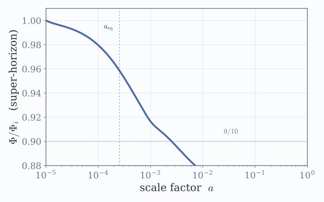
Superhorizon evolution of \(\Phi\) for a fixed \(k=10^{-4}\,\mathrm{Mpc^{-1}}\) mode that never enters the horizon (Baumann Fig. 6.3). Constant deep in radiation domination, constant again deep in matter domination, and dropping by exactly the predicted \(9/10\) through the transition at \(a_{\rm eq}\).
That \(9/10\), computed by nothing more than reading off Φ(p, a) at early and late times, is the whole content of the "curvature perturbation is conserved on superhorizon scales" statement often quoted without the caveat — it's conserved between constant-\(w\) eras, not straight through a transition.
Radiation domination and the Mészáros effect
Before equality, radiation — not matter — dominates \(\bar\rho\) and hence \(H\) and \(\Psi\). A CDM mode that enters the horizon during radiation domination still obeys \(\ddot\delta_c+2H\dot\delta_c=4\pi G\bar\rho_m\delta_m\big|_{\rm source}\), but now the friction term \(2H\dot\delta_c\) is enormous (radiation-era \(H\) is much larger than matter alone would give) while the source on the right is small (CDM is a minority species, and the majority radiation component doesn't clump — it just oscillates as an acoustic wave, stabilised by its own pressure). Friction wins: subhorizon CDM growth nearly stalls, growing only logarithmically in \(a\) instead of linearly — the Mészáros effect. Once the universe crosses into matter domination at \(a_{\rm eq}\), the source term catches up, friction and gravity rebalance, and \(\delta_c\propto a\) resumes.
The mechanism is visible directly in the potential itself: unlike the superhorizon case above, a mode that enters the horizon during radiation domination doesn't just sit at a new constant value — the \(k^2\Phi\) term switches on, \(\Phi\) starts oscillating with the acoustic wave, and its amplitude decays as \(a^{-2}\). That collapsing potential is exactly the "source" that goes missing from the CDM growth equation above:
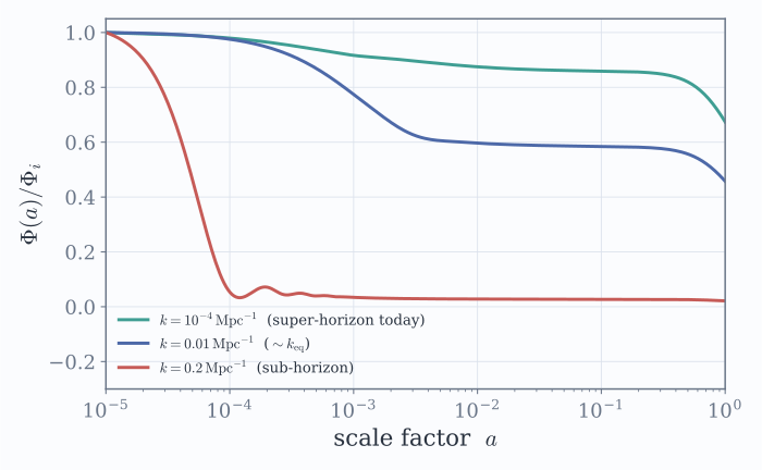
\(\Phi(a)\) for three modes (Baumann Fig. 6.5). The super-horizon mode barely moves before today; the \(k\sim k_{\rm eq}\) mode drops partway through horizon crossing near equality; the deeply sub-horizon mode enters during radiation domination and collapses almost to zero, oscillating and decaying as \(a^{-2}\) along the way — precisely the mechanism starving CDM growth of its source term in the Mészáros effect.
The net effect on matter is a permanent suppression of small-scale clustering relative to large scales: modes that entered the horizon early (small \(k^{-1}\), deep in radiation domination) spent longer being starved than modes that entered late (large \(k^{-1}\), near or after equality). That is precisely what builds the characteristic bend in the matter power spectrum at the scale corresponding to the horizon size at equality, \(k_{\rm eq}=\mathcal H(a_{\rm eq})\) — plotted below, straight out of Cosmic.jl.
Verifying with Cosmic.jl
solve_perturbations integrates the full system above — the coupled Einstein and fluid/Boltzmann equations, one Fourier mode \(k\) at a time — for photons, neutrinos, baryons and cold dark matter simultaneously:
julia> using Cosmic

julia> c = cosmology(); rec = recombination(c);

julia> p = solve_perturbations(c, rec, 0.2);   # one sub-horizon Fourier mode, k = 0.2 / Mpc

julia> δ_cdm(p, 1.0), δ_baryon(p, 1.0)         # CDM and baryon contrast today, same k
(-24327.3, -24199.0)
Two things worth noticing already: both are large and negative (this mode has been growing since long before today, and the sign is a normalisation convention — \(\delta\) is defined relative to a positive primordial curvature perturbation), and \(\delta_{\rm cdm}\approx\delta_{\rm baryon}\) to within half a percent. That near-equality is itself a result worth checking, not an assumption: right at recombination (Part 4) this same mode has \(\delta_{\rm baryon}\) at barely \(2\%\) of \(\delta_{\rm cdm}\) — Thomson-coupled to the photons until then, baryons couldn't fall into CDM's potential wells at all. Once the photons let go, gravity pulls the baryon distribution into agreement with the (by then much better-developed) CDM one, and by today the two are nearly identical.
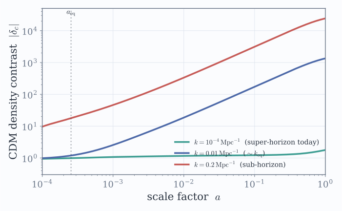
The CDM density contrast \(\delta_c(a)\) for three Fourier modes (Baumann Fig. 6.6), all normalised to the same primordial curvature perturbation. The large-scale mode (still outside the horizon today) barely grows at all; the two smaller-scale modes, already sub-horizon well before equality, grow at a measurably reduced rate near \(a_{\rm eq}\) (locally \(\delta\propto a^{0.7}\), not \(a^1\)) — the Mészáros suppression — before both settle onto the full \(\delta\propto a\) growing-mode slope through the bulk of matter domination. The curves stay offset from each other throughout (smaller scales carry more power, not the same value), and all three growth rates fall again once dark energy takes over near \(a\sim0.5\).
Adding baryons and photons. Follow one representative sub-horizon mode a step further and track all three species at once — dark matter, baryons and photons — rather than dark matter alone:
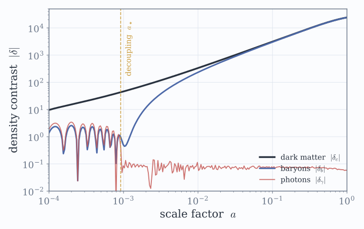
\(|\delta_c|\), \(|\delta_b|\), \(|\delta_\gamma|\) for one sub-horizon mode (Baumann Fig. 6.8). All three start comparable in size. Before decoupling the baryons are Thomson-coupled to the photons and oscillate in lock-step with them — the baryon acoustic oscillations of Part 4, seen here in the density contrast itself rather than in the CMB. Dark matter, immune to photon pressure, ignores the oscillation entirely and grows smoothly (with the Mészáros-suppressed slope derived above). The instant photons decouple, baryons lose their pressure support, stop oscillating, and fall straight into the potential wells CDM had a head start building — the dip-and-recovery right at \(a_\star\) — catching back up to \(\delta_c\) by today.
The growth factor and growth rate. \(D(a)=\delta_m(a)/\delta_m(1)\) is normalised to \(1\) today and falls monotonically into the past. Its logarithmic slope, \(f\equiv\mathrm d\ln D/\mathrm d\ln a\), is the more diagnostic quantity: for the pure power law \(D\propto a\) derived above, \(f=1\) exactly, and departures from \(f=1\) are a direct, scale-independent measurement of how much the growth law has bent away from matter domination — which is exactly why redshift-space-distortion surveys report \(f\) rather than \(D\) itself. In \(\Lambda\)CDM \(f\) is famously close to \(\Omega_m(a)^{0.55}\):
julia> growth_factor(c, rec, 0.0)              # D(z), normalised to D(0) = 1 by definition
1.0

julia> growth_rate(c, rec, 0.0)                # f = dlnD/dlna, today
0.51604

julia> Ω_m(c)^0.55                             # the textbook approximation f ≈ Ω_m(a)^0.55
0.52480
Less than 2% apart — the approximation earns its textbook status. (One honest caveat: growth_factor's default \(k=10^{-3}\,\mathrm{Mpc^{-1}}\) is a genuinely enormous scale, comparable to today's horizon, so it is still marginally outside the horizon at very early times; on those largest scales \(\delta_m\) picks up relativistic corrections beyond the simple Newtonian-gauge picture, which is exactly the gauge subtlety flagged above — Cosmic.jl's own docs point you to δ_matter_comoving for the textbook super-horizon behaviour instead.)
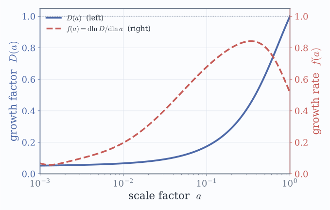
Left axis: the growth factor \(D(a)\), climbing from near zero to \(1\) today. Right axis: the growth rate \(f(a)=\dd\ln D/\dd\ln a\), which rises through matter domination — approaching, but not quite reaching, the matter-domination value \(f=1\), a reminder that even this large a scale never sits in a perfectly clean matter-only regime — then turns over and falls once dark energy starts suppressing growth, landing at \(f\simeq0.52\) today.
The matter power spectrum. matter_power_spectrum runs the Boltzmann hierarchy over a grid of \(k\) and assembles \(P(k)\); transfer and power read it off, and σ8 is the headline number every large-scale-structure survey quotes:
julia> P = matter_power_spectrum(c, rec);

julia> σ8(P)                                    # RMS matter fluctuation in 8/h Mpc spheres
0.8143

julia> power(P, 0.01), power(P, 1.0)            # P(k) in Mpc³, large scale vs small scale
(80081.5, 90.4)
\(\sigma_8=0.814\) is within a percent of Planck's measured \(0.811\pm0.006\) — from a species list and the derivation above, no fitting involved. And \(P(k)\) itself has fallen by three orders of magnitude between \(k=0.01\) and \(k=1\,\mathrm{Mpc^{-1}}\), the small-scale suppression the Mészáros effect predicts, now visible in the full spectrum rather than one mode at a time.
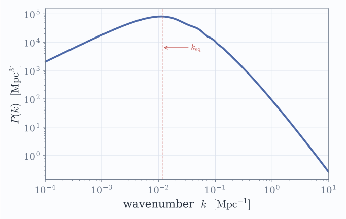
The linear matter power spectrum \(P(k)\) from Cosmic.jl. Large scales (\(k\ll k_{\rm eq}\)) preserve the primordial slope; small scales (\(k\gg k_{\rm eq}\)) are suppressed by the Mészáros effect derived above, bending the spectrum over at \(k_{\rm eq}\) — the comoving horizon scale at matter–radiation equality. (This grid is coarse enough to miss them, but a finer one shows baryon acoustic oscillations riding on top — the same sound waves whose frozen imprint set \(r_{\rm drag}\) in Part 4.)
Where does that headline \(\sigma_8\) number actually come from? Not from \(P(k)\) directly — from the dimensionless spectrum \(\Delta^2(k)\equiv k^3P(k)/2\pi^2\), the power per logarithmic interval in \(k\), smoothed with a top-hat window of comoving radius \(R\) and integrated:
\[ \sigma^2(R) = \int \mathrm d\ln k\;\Delta^2(k)\,W^2(kR) . \]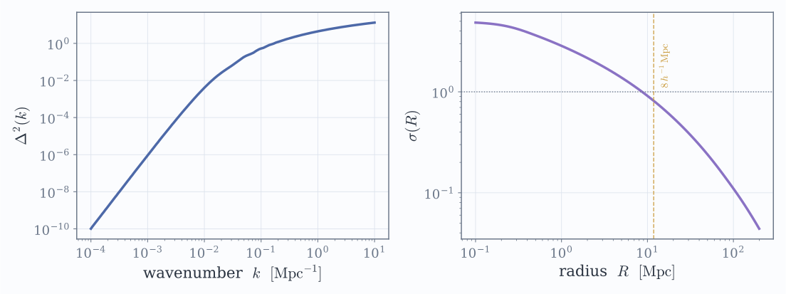
Left: \(\Delta^2(k)\) (Baumann Fig. 5.5) — the same bend at \(k_{\rm eq}\), now per logarithmic interval. Right: \(\sigma(R)\), monotonically falling as the smoothing scale grows — bigger spheres average over more structure and fluctuate less. \(\sigma_8\) is just this curve read off at \(R=8\,h^{-1}\,\mathrm{Mpc}\) (dashed), which is why the two panels are really one calculation: σ8(P) is σ_R(P, 8/h) under the hood.
Where we are
Five posts ago we started from two words, homogeneous and isotropic, and derived a background universe that Cosmic.jl reproduces to the percent level. This post broke that symmetry: perturbing the metric and the matter, first Newtonian then fully relativistic, gives a single gravitational instability equation that — depending on horizon crossing and which era it happens in — either grows as \(a\), stalls logarithmically, or oscillates as a sound wave. That one piece of physics, run forward from a near-scale-invariant primordial spectrum to today, is the entire origin story of every galaxy, cluster, and filament in the observable universe.
What we still haven't touched is where the primordial perturbations came from (inflation, Baumann Ch. 8), or the detailed physics of the CMB anisotropies themselves — the acoustic peaks, polarisation, and the Boltzmann-equation treatment of the photon-baryon fluid before recombination (Ch. 7) — both of which Cosmic.jl also computes in full, via cmb_spectra and inflaton_spectrum. Those are posts for another day.
← Back to the course overview.