
The Expanding Universe I — Geometry
Part 1 of a four-part reading of Baumann's Chapter 2. Before we can ask how fast the universe expands, we have to ask what its shape is. We will derive — not just quote — the metric of the cosmos, and find that two symmetry assumptions leave essentially no freedom at all.
This is the first of five connected posts — Geometry, Kinematics, Dynamics, Our Universe, Perturbations — that build the universe from the ground up, from perfect homogeneity to the structure that grows on top of it, and check every result against my Julia package Cosmic.jl.
The cosmological principle
Cosmology becomes a science once we make one bold simplification, promoted to a principle:
Isotropy about every point already implies homogeneity, and the two together are a severe constraint. A general spacetime needs ten functions \(g_{\mu\nu}(x)\) of four coordinates; we are about to see homogeneity and isotropy grind that down to one function of time and one constant.
In GR the geometry lives in the line element \(\mathrm d s^2 = g_{\mu\nu}\mathrm d x^\mu\mathrm d x^\nu\), and proper time follows from \(c^2\mathrm d\tau^2=-\mathrm d s^2\). Because the universe can be sliced into homogeneous "now" surfaces stacked along a cosmic time \(t\), the metric must take the form
\[ \mathrm d s^2 = -c^2\mathrm d t^2 + a^2(t)\,\mathrm d\ell^2 ,\]with \(a(t)\) the scale factor and \(\mathrm d\ell^2\) the metric of a fixed, maximally symmetric 3-space. Finding \(\mathrm d\ell^2\) is the whole geometric problem, so let us derive it.
Symmetric three-spaces — derived from an embedding
What are the homogeneous, isotropic 3-geometries? The trick is to realise a curved 3-space as a surface inside a flat 4-space. Take Euclidean coordinates \((\mathbf x,u)=(x_1,x_2,x_3,u)\) and impose
\[ \mathbf x^2 \pm u^2 = \pm R_0^2 , \qquad \mathrm d\ell^2 = \mathrm d\mathbf x^2 \pm \mathrm d u^2 ,\]where the upper sign carves out a 3-sphere (radius \(R_0\), positive curvature) and the lower sign a 3-hyperboloid (negative curvature). The flat case is the limit \(R_0\to\infty\).
We want to eliminate the auxiliary coordinate \(u\). Differentiate the constraint:
\[ 2\,\mathbf x\cdot\mathrm d\mathbf x \pm 2u\,\mathrm d u = 0 \;\Longrightarrow\; \mathrm d u = \mp\frac{\mathbf x\cdot\mathrm d\mathbf x}{u}, \qquad \mathrm d u^2 = \frac{(\mathbf x\cdot\mathrm d\mathbf x)^2}{u^2}. \]From the constraint \(u^2 = \pm(R_0^2 - \mathbf x^2)\cdot(\pm1)=\,\)… more usefully, \(\pm u^2 = \pm R_0^2 - \mathbf x^2\), i.e. \(u^2 = R_0^2 \mp \mathbf x^2\) for the two cases. Substituting,
\[ \pm\mathrm d u^2 = \pm\frac{(\mathbf x\cdot\mathrm d\mathbf x)^2}{R_0^2 \mp \mathbf x^2}. \]Introduce \(k=+1\) for the sphere and \(k=-1\) for the hyperboloid so the two signs merge. Then \(\mathrm d\ell^2 = \mathrm d\mathbf x^2 \pm\mathrm d u^2\) becomes the single formula
\[ \boxed{\;\mathrm d\ell^2 = \mathrm d\mathbf x^2 + k\,\frac{(\mathbf x\cdot\mathrm d\mathbf x)^2}{R_0^2 - k\,\mathbf x^2}\;}, \qquad k=\begin{cases}+1 & \mathrm S^3 \text{ (closed)}\\ \ 0 & \mathrm E^3 \text{ (flat)}\\ -1 & \mathrm H^3 \text{ (open)}\end{cases}\]with \(k=0\) (flat) recovered as the \(R_0\to\infty\) limit. Now switch to spherical polar coordinates \((r,\theta,\phi)\). Using
\[ \mathrm d\mathbf x^2 = \mathrm d r^2 + r^2\mathrm d\Omega^2, \qquad \mathbf x\cdot\mathrm d\mathbf x = r\,\mathrm d r, \qquad \mathbf x^2 = r^2, \](with \(\mathrm d\Omega^2\equiv\mathrm d\theta^2+\sin^2\theta\,\mathrm d\phi^2\)) the messy term collapses and
\[ \boxed{\;\mathrm d\ell^2 = \frac{\mathrm d r^2}{1 - k\,r^2/R_0^2} + r^2\,\mathrm d\Omega^2.\;}\]The Robertson–Walker metric
Substituting this spatial metric back into the spacetime line element gives the Robertson–Walker (RW) metric, the geometry of any homogeneous, isotropic universe:
\[ \boxed{\;\mathrm d s^2 = -c^2\mathrm d t^2 + a^2(t)\left[\frac{\mathrm d r^2}{1 - k\,r^2/R_0^2} + r^2\mathrm d\Omega^2\right].\;}\]Ten functions have become one function of time \(a(t)\) and one constant \(R_0\) (with \(k\) its sign). That is the complete geometric content of the cosmos — symmetry did the rest.
A rescaling freedom. The line element is invariant under \(a\to\lambda a,\ r\to r/\lambda,\ R_0\to R_0/\lambda\). We spend this freedom to set \(a(t_0)\equiv1\) today; then \(R_0\) is the physical curvature radius now, justifying its subscript.
Comoving versus physical. The coordinate \(r\) is comoving: it labels a galaxy and does not change as space stretches. The physical distance is \(r_{\rm phys}=a(t)\,r\). Differentiate to get the velocity of a galaxy at fixed comoving position plus a peculiar drift \(\dot{\mathbf r}\):
\[ \mathbf v_{\rm phys} = \frac{\mathrm d\mathbf r_{\rm phys}}{\mathrm d t} = \dot a\,\mathbf r + a\,\dot{\mathbf r} = \underbrace{\frac{\dot a}{a}\,\mathbf r_{\rm phys}}_{\text{Hubble flow}} + \underbrace{a\,\dot{\mathbf r}}_{\text{peculiar}} ,\]which defines the Hubble parameter
\[ \boxed{\;H \equiv \frac{\dot a}{a}.\;}\]The first term is pure recession from the stretching of space; the second is the galaxy's own motion. A comoving observer has \(\dot{\mathbf r}=0\), and cosmic time \(t\) is the time on their clock.
Deriving \(S_k(\chi)\): the metric distance
The factor \(1/(1-kr^2/R_0^2)\) is inconvenient, so define a new radial coordinate that absorbs it:
\[ \mathrm d\chi \equiv \frac{\mathrm d r}{\sqrt{1 - k\,r^2/R_0^2}} . \]Integrating for each sign of \(k\) inverts to give \(r\) as a function of \(\chi\). For \(k=+1\), \(\int\mathrm d r/\sqrt{1-r^2/R_0^2}=R_0\arcsin(r/R_0)=\chi\), so \(r=R_0\sin(\chi/R_0)\); for \(k=-1\) the arcsine becomes \(\mathrm{arcsinh}\); for \(k=0\), \(r=\chi\). Collecting all three, the metric becomes
\[ \mathrm d s^2 = -c^2\mathrm d t^2 + a^2(t)\big[\mathrm d\chi^2 + S_k^2(\chi)\,\mathrm d\Omega^2\big], \qquad S_k(\chi) = R_0\begin{cases}\sin(\chi/R_0) & k=+1\\ \chi/R_0 & k=0\\ \sinh(\chi/R_0) & k=-1\end{cases}\]The metric distance \(S_k(\chi)\) is what carries the curvature into every observable in the next post. Its three shapes are the entire freedom the geometry has:
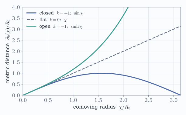
The metric distance \(S_k(\chi)\) for the three geometries. In a closed universe (\(k=+1\)) distances grow more slowly than \(\chi\) and eventually turn back on themselves (\(\sin\)); in a flat one they grow linearly; in an open one they run away (\(\sinh\)). We will feed these three cases straight into Cosmic.jl in Parts 2 and 3 and watch them reshape the observable distances and the fate of the universe.
Conformal time
One last change of variables. Define conformal time \(\eta\) by
\[ \boxed{\;\mathrm d\eta = \frac{\mathrm d t}{a(t)}\;} \quad\Longrightarrow\quad \mathrm d s^2 = a^2(\eta)\big[-c^2\mathrm d\eta^2 + \mathrm d\chi^2 + S_k^2(\chi)\mathrm d\Omega^2\big].\]The metric factorises into a static piece times an overall \(a^2(\eta)\). The reason this is so useful: radial light rays (\(\mathrm d s^2=0\), \(\mathrm d\Omega=0\)) obey \(\mathrm d\chi = \pm c\,\mathrm d\eta\) — straight 45° lines in the \((\chi,\eta)\) plane, exactly as in special relativity. The comoving distance a photon covers is simply the elapsed conformal time. Every causal question — horizons, how far light has travelled since the Bang — is read off most cleanly in \(\eta\).
Verifying with Cosmic.jl
Geometry alone does not fix \(a(t)\); that waits for the Friedmann equations in Part 3. But once Cosmic.jl has the expansion history of our real universe, the two functions we just introduced — \(a(t)\) and \(\eta(a)\) — are one call each.
julia> using Cosmic

julia> c = cosmology();          # Planck 2018 ΛCDM, spatially flat

julia> age(c)                    # the age of the universe, in billions of years
13.787

julia> scale_factor_of_time(c, age(c))   # a is 1 today, by our convention
1.0

julia> conformal_time_today(c)   # the comoving horizon today, in Mpc
14165.2

julia> hubble_distance(c)        # the Hubble distance c/H₀, in Mpc
4430.87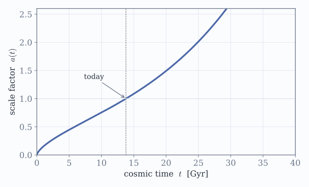
The scale factor of our universe, integrated by Cosmic.jl. It starts at \(a=0\) (the Big Bang), rises with a decelerating slope while matter pulls back, then inflects upward in the last few billion years as dark energy takes over. By the rescaling freedom, \(a=1\) at the present age — and Cosmic returns exactly that.
The comoving horizon. Conformal time is not just a coordinate trick — \(\eta(a)\) measured in Mpc is the comoving distance light has travelled since \(a'=0\), the particle horizon. Because it is dominated by early times, most of the horizon was laid down long ago and late-time expansion adds little:
julia> conformal_time(c, 1e-3)   # comoving horizon back near recombination, in Mpc
299.5

julia> conformal_time(c, 1.0)    # comoving horizon today, in Mpc
14165.2
So the comoving size of the observable universe has grown by roughly \(14165/300 \approx 47\) times since last scattering.
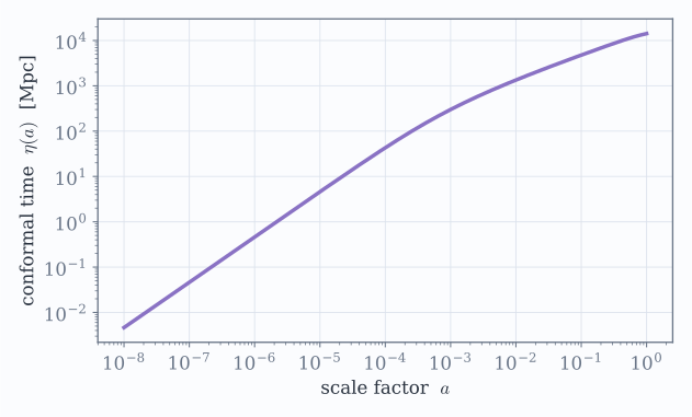
The comoving horizon \(\eta(a)=\int_0^a \dd a'/(a'^2H)\) accumulating as the universe expands (log–log). The curve flattens: once dark energy dominates, the comoving horizon barely grows, and distant galaxies slip permanently out of causal reach. Computed with conformal_time(c, a).
The curvature radius. For a curved universe, \(R_0\) is finite and Cosmic carries it through the curvature parameter \(\Omega_k\equiv-kc^2/(R_0H_0)^2\). We can read off the physical curvature radius today directly:
julia> c_open = cosmology(Ω_c = 0.25, Ω_k = 0.05);   # a mildly open universe

julia> Ω_k(c_open)               # the curvature density parameter
0.05

julia> hubble_distance(c_open) / sqrt(abs(Ω_k(c_open)))   # curvature radius R₀, in Mpc
19815.8
We will put \(\Omega_k\) to real work in Part 2, where the sign of \(k\) — the choice of \(\sin\), \(\chi\) or \(\sinh\) in \(S_k\) — visibly bends the distance–redshift relation, and again in Part 3, where it decides whether the universe expands forever or recollapses.
Where we are
Two symmetry assumptions, one embedding, and a couple of coordinate changes gave us the Robertson–Walker metric: a single scale factor \(a(t)\), a curvature constant \(k\), and the tools \(\chi\), \(S_k(\chi)\) and \(\eta\). We have the stage. In Part 2 — Kinematics we release light and free particles onto it and derive redshift and the several distances of cosmology.