
Renormalisation Group IV: Fixed Points and Universality
Part 4 of eight. previous: Block spins · Course home · Glossary · next: Wilson's shells
A line of spins never becomes a magnet. A flat sheet of spins does: below a critical temperature \(T_c\) most of them line up. Right at \(T_c\) something strange happens and this part is about what.
What a critical point looks like
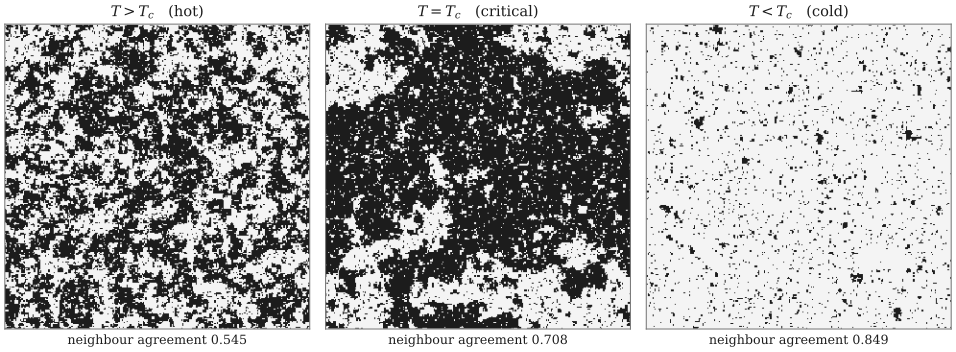
Three snapshots of a simulated 256×256 Ising magnet, with how often neighbouring spins agree printed underneath. Hot: small islands, short-range order. Cold: one colour nearly everywhere. Critical: islands inside lakes inside islands, at every size up to the whole box, with the agreement sitting at the exact value \(1/\sqrt2=0.707\).
At \(T_c\) there is no typical size of island. There are small ones, medium ones and huge ones, all at once. In the language of Part 3, the correlation length is infinite.
Near \(T_c\) the correlation length follows a power law,
\[ \xi \propto |T-T_c|^{-\nu}, \]and other quantities do too. The heat capacity goes like \(|T-T_c|^{-\alpha}\), the magnetisation below \(T_c\) like \((T_c-T)^{\beta}\) and the magnetic susceptibility like \(|T-T_c|^{-\gamma}\). (The susceptibility \(\chi=\partial m/\partial h\) is just how much magnetisation you get for a small applied field: near \(T_c\) a feather touch produces a big response, which is why it diverges.) The numbers \(\nu,\alpha,\beta,\gamma\) are called critical exponents. Before the RG, two facts about them were a complete mystery:
They are usually not simple fractions. For a 3D magnet, \(\nu=0.6300\) and \(\beta=0.3265\). Nothing in the energy formula looks anything like these numbers. Tong suggests thinking of them as new mathematical constants, like \(\pi\) or \(e\), only more subtle.
They are universal. A magnet, the liquid-gas critical point of water and a metal alloy sorting itself onto its lattice all have the same exponents, even though the atoms involved have nothing in common.
Both facts come from one picture.
Why the critical point is a fixed point
Recall the rule from Part 3: one coarse-graining step with scale factor \(b\) changes the couplings, \(K\to K'\) and divides the correlation length (in lattice units) by \(b\). At \(T_c\), \(\xi=\infty\) and \(\infty/b\) is still \(\infty\). So the critical point flows to a point with infinite correlation length and that has to be a fixed point \(K^*\). It can't be \(K=0\) or \(K=\infty\), where \(\xi=0\). It's a genuinely new fixed point.
You can see this directly by coarse-graining the snapshots:
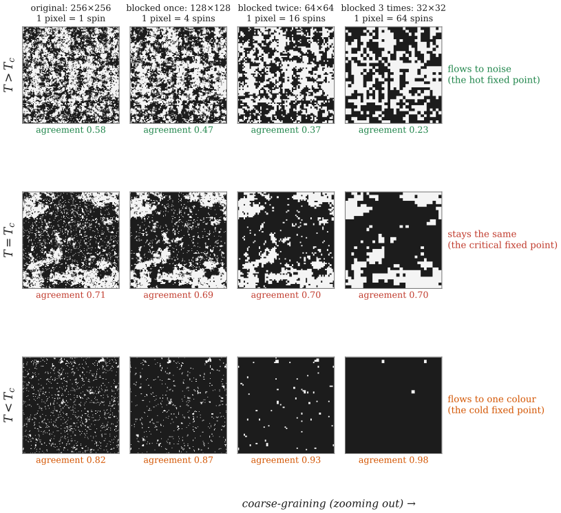
Three rounds of 2×2 majority voting, with the neighbour agreement printed under each panel (averaged over 16 independent simulations). Hot (top row): the picture flows towards noise, the \(K=0\) fixed point, with the number falling from 0.58 to 0.23. Cold (bottom row): it flows to one colour, the \(K=\infty\) fixed point, with the number climbing from 0.82 to 0.98. At \(T_c\) (middle row) the number stays near \(1/\sqrt2=0.707\), the exact Ising value: that is the new fixed point. For the critical row the picture shown is a sample with a small net magnetisation, so both colours are visible; the numbers come from the unbiased set of samples.
Now try it live. This simulation runs in your browser:
Set \(T/T_c=1.05\) and watch. The first panel still looks roughly critical, but by the third blocking the noise has won. Move to \(0.97\) and the opposite happens. The closer you are to \(T_c\), the more blocking steps it takes before you can tell which way the flow is going. That delay is the long correlation length, seen through the RG.
Linearising the flow: relevant and irrelevant
Near a fixed point, small deviations grow or shrink by the same factor at every step. With one coupling, write \(K=K^*+\delta K\) and expand the map to first order:
\[ \delta K' = R'(K^*)\,\delta K \;\equiv\; b^{\,y}\,\delta K. \](The slope \(R'(K^*)\) is written as \(b^{y}\) because that is the only form that survives doing two steps in a row: two steps of size \(b\) must equal one step of size \(b^2\) and \(b^yb^y=(b^2)^y\). Note this \(b\) is the zoom factor, nothing to do with the cutoff \(\Lambda\) of Parts 1 and 2.)
There are three cases:
Temperature has to be relevant at a critical point, because being slightly off \(T_c\) is exactly what makes the system flow away. Write \(t=(T-T_c)/T_c\) and call its exponent \(y_t\). Since coarse-graining divides lengths by \(b\) and multiplies \(t\) by \(b^{y_t}\),
\[ \xi(t) = b\,\xi(b^{y_t}t). \]This works for any \(b\), so choose \(b=|t|^{-1/y_t}\), which makes the argument on the right equal to \(\pm1\):
\[ \xi(t) = |t|^{-1/y_t}\,\xi(\pm1) \quad\Longrightarrow\quad \boxed{\;\nu = \frac1{y_t}.\;} \]A critical exponent is one over the growth rate of the flow near the fixed point. It belongs to the fixed point, not to the atoms you started with. That's why \(\nu\) doesn't have to be a nice fraction: it's whatever the slope of a complicated map happens to be.
Many couplings and universality
Real coarse-graining creates new couplings: bonds between next-nearest neighbours, four-spin terms and so on. So the RG really acts on an enormous space of couplings \(\{K_1,K_2,\dots\}\), which Tong calls "theory space". Near a fixed point you linearise just as before. Each independent direction comes with its own \(b^{y_i}\).
The crucial fact is that only a few directions are relevant. For the Ising fixed point there are exactly two: temperature \(t\) and magnetic field \(h\). The infinitely many others are all irrelevant.
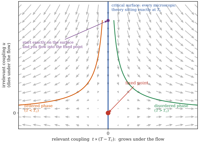
The flow near a fixed point, with one relevant coupling across and one irrelevant one up. The critical surface (blue line) is every starting theory that flows into the fixed point. Start slightly off it and you first head towards the fixed point, then peel away to one phase or the other.
The irrelevant directions make up the critical surface: the set of all microscopic systems that are exactly critical. A real magnet, with its messy crystal structure, sits somewhere on this surface when it's tuned to \(T_c\). So does a liquid at its critical point, once you match up "density" with "magnetisation". Under the flow they all slide into the same fixed point and forget everything about where they started except the relevant directions.
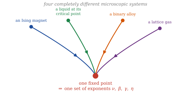
Four very different systems flowing to one fixed point. The exponents belong to the destination, so everything that arrives there shares them.
This is universality. Two systems are in the same universality class when they flow to the same fixed point. Measurements on fluids such as xenon and sulfur hexafluoride near their critical points give \(\beta\approx0.32\) to \(0.33\), matching the 3D Ising value of \(0.3265\).
It also explains why reaching a critical point needs exactly two knobs, temperature and field: you need one knob per relevant direction. As Tong points out, an experimenter can easily turn the thermostat, but has no knob for the \(\phi^4\) strength or the next-neighbour bonds. Luckily those are irrelevant, so nobody needs to tune them.
All the exponents from two numbers
Here's a simple way to see why exponents are linked. Near \(T_c\), the spins inside one correlation length move together, like one coherent block (Tong's picture). In a box of size \(L\) there are \((L/\xi)^d\) such blocks and each one carries roughly the same free energy. So the free energy per site scales like \(\xi^{-d}\propto|t|^{d\nu}\). Its second derivative, the heat capacity, then goes like \(|t|^{d\nu-2}\), which gives \(\alpha=2-d\nu\).
To make this exact, follow the free energy through one RG step. After the step, each new site stands for a block of \(b^d\) old sites and the total free energy doesn't change (coarse-graining keeps the physics). So the free energy per site before the step is \(b^{-d}\) times the free energy per site after it and after the step \(t\) and \(h\) have become \(b^{y_t}t\) and \(b^{y_h}h\). That gives
\[ f(t,h) = b^{-d}\,f(b^{y_t}t,\ b^{y_h}h), \]and taking derivatives gives every exponent in terms of \(y_t\) and \(y_h\) (exercise 4.2 derives \(\beta\)):
\[ \nu=\frac1{y_t},\quad \alpha = 2-\frac{d}{y_t},\quad \beta=\frac{d-y_h}{y_t},\quad \gamma=\frac{2y_h-d}{y_t},\quad \delta=\frac{y_h}{d-y_h},\quad \eta=d+2-2y_h. \]Six exponents from two numbers means four relations between them and they hold automatically:
\[ \alpha+2\beta+\gamma=2\ \ (\text{Rushbrooke}),\qquad \gamma=\beta(\delta-1)\ \ (\text{Widom}),\qquad \gamma=\nu(2-\eta)\ \ (\text{Fisher}),\qquad d\nu=2-\alpha\ \ (\text{Josephson}). \]Experimenters found these relations before anyone could explain them. Checking them in Wolfram:
al = 2 - d/yt; be = (d - yh)/yt; ga = (2 yh - d)/yt;
de = yh/(d - yh); nu = 1/yt; eta = d + 2 - 2 yh;
Simplify[{al + 2 be + ga - 2, ga - be (de - 1), ga - nu (2 - eta), d nu - (2 - al)}]
(* {0, 0, 0, 0} *)
{nu, al, be, ga, de, eta} /. {d -> 2, yt -> 1, yh -> 15/8}
(* {1, 0, 1/8, 7/4, 15, 1/4}  : Onsager's exact 2D Ising exponents *)
For the 2D Ising model, Onsager's exact solution corresponds to \(y_t=1\) and \(y_h=15/8\).
Finding the 2D critical temperature
A mirror trick gives it exactly
Das (§15.4) shows a beautiful argument due to Kramers and Wannier. The 2D Ising partition function at a hot coupling \(K\) can be rewritten exactly as the partition function at a cold coupling \(K^*\), where
\[ \sinh 2K\,\sinh 2K^* = 1. \]On the mirror, \(K=K^*\), so \(\sinh^2 2K_c=1\), which gives \(K_c=\tfrac12\ln(1+\sqrt2)=0.4407\). (Wolfram: Solve[Sinh[2 K]^2 == 1 && K > 0, K, Reals] gives \(\tfrac12\operatorname{arsinh}1 = 0.440687\).) This is the exact answer, but the trick only tells you where the transition is, not its exponents.
A rough RG recursion gets the structure
Can we get the exponents with a pencil? Not exactly, because majority voting in 2D creates infinitely many couplings. The simplest approximation that keeps just one coupling is the Migdal-Kadanoff scheme. On the square lattice with \(b=2\), first move half the bonds onto their neighbours, which leaves one-dimensional chains with doubled coupling \(2K\). Then decimate those chains exactly as in Part 3. The result is
\[ K' = \operatorname{artanh}\!\big(\tanh^2 2K\big) = \tfrac12\ln\cosh 4K. \]Unlike the 1D map, this one crosses the diagonal:
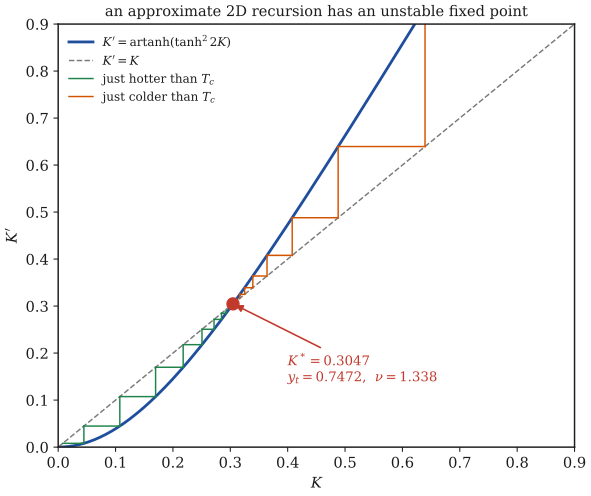
Start a tiny step to either side of \(K^*\) and the steps run away in opposite directions, to the hot fixed point or the cold one. So \(K^*\) is a fixed point where temperature is relevant: a phase transition.
Solving numerically (with Wolfram's FindRoot and checked in Python and JavaScript): \(K^*=0.3047\), \(R'(K^*)=1.6786\), so \(y_t=\log_2 1.6786=0.7472\) and \(\nu=1.338\).
Compare with the exact answers: \(K_c=0.4407\) and \(\nu=1\). The rough scheme gets the structure right (there is a fixed point and temperature is relevant there) but the numbers are off by about 30%.
You could live with 30%. Finding out about it is the harder part, because bond moving is not the first term of anything. There is no second term to compute, no small quantity being expanded, so no way to put an error bar on the answer without already knowing it. A number with no error bar is still a guess, however confident it looks.
There are better ways to get the numbers. One is to solve the model exactly, which Onsager managed in 1944. That works for this model alone. Another is Wilson's momentum-space method, which has a genuinely small quantity to expand in: that is Parts 5 and 6. The third is to measure the exponents by simulating the model, which is where the rest of this part goes, because it runs on exactly the scaling laws built above.
Measuring the exponents
The trick: at \(T_c\), the box itself is the ruler
Away from \(T_c\) the correlation length \(\xi\) is finite, so a simulation in a box of side \(L\) behaves like the infinite system as long as \(L\gg\xi\). At \(T_c\) that breaks down, because \(\xi\) is infinite. There is then nothing left to set a scale except \(L\) itself, so every quantity has to be a pure power of \(L\). That is the scaling hypothesis of this part with the rescaling factor \(b\) replaced by the box size, so the powers that show up are the same exponents.
This gives three measurements, from the same simulation.
1. Where \(K_c\) is: the Binder cumulant. Build the dimensionless ratio
\[ U=1-\frac{\langle m^4\rangle}{3\,\langle m^2\rangle^2}. \]2. How fast the flow runs: the slope at the crossing. Off the critical point, \(U\) depends on \(L\) only through the combination \(L/\xi\sim L\,|t|^{\nu}\), so \(U\) is a function of \(L^{1/\nu}t\). Differentiating in \(t\) at the crossing brings down one factor of \(L^{1/\nu}\):
\[ \left.\frac{\mathrm d U}{\mathrm d K}\right|_{K_c}\propto L^{1/\nu}. \]So the slopes of those curves, plotted against \(L\) on log axes, give \(1/\nu\) as a straight line. No approximation has been made anywhere.
3. The other exponents. The same argument on the susceptibility and the magnetisation at \(K_c\):
\[ \chi\big|_{K_c}\propto L^{\gamma/\nu},\qquad \langle|m|\rangle\big|_{K_c}\propto L^{-\beta/\nu}. \]What comes out
The simulations use the Wolff cluster algorithm, because near \(T_c\) flipping one spin at a time is hopelessly slow. Seven box sizes from \(L=8\) to \(L=64\), thirteen temperatures around \(K_c\), eight independent chains at each point with 30,000 measurements per chain. That is a few core-hours on a shared machine, small enough to repeat on a laptop.
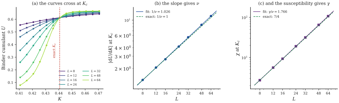
(a) The Binder cumulant for seven box sizes. Away from \(K_c\) the curves fan out, at \(K_c\) they pass through one point, which is the dashed line at the exact answer. Nothing was fitted to put it there. (b) The slope of those curves at \(K_c\), against \(L\). The straight line has gradient \(1/\nu\). (c) The susceptibility at \(K_c\), whose gradient is \(\gamma/\nu\).
The crossings march towards the exact value as the boxes grow:
| pair \((L,2L)\) | crossing \(K_\times\) |
|---|---|
| \((8,16)\) | 0.44182 |
| \((12,24)\) | 0.44111 |
| \((16,32)\) | 0.44104 |
| \((24,48)\) | 0.44083 |
| \((32,64)\) | 0.44076 |
| exact | 0.440687 |
Collecting everything, side by side with the pencil method:
| Migdal-Kadanoff | measured here | exact | |
|---|---|---|---|
| \(K_c\) | 0.3047, off by \(-31\%\) | \(0.44076\pm0.00008\), off by \(+0.02\%\) | 0.440687 |
| \(\nu\) | 1.338, off by \(+34\%\) | \(0.96\pm0.04\), off by \(-4\%\) | 1 |
| \(\gamma/\nu\) | not available | \(1.763\pm0.005\) | 1.75 |
| \(\beta/\nu\) | not available | \(0.128\pm0.002\) | 0.125 |
| \(U\) at \(K_c\) | not available | \(0.6101\pm0.0006\) | 0.61069 |
Notice what has not happened here. Nobody worked out a recursion for \(K\), nobody had to guess which couplings to keep, nobody moved a bond. The scaling laws of this part were assumed, then the exponents in them were measured. That the answers come out at the exact values is a test of the RG picture itself, not of any particular approximation scheme.
That said, measurement alone does not explain why a magnet and a boiling liquid share these numbers. For that we still need a fixed point we can actually calculate at, which is what Wilson's momentum-space method gives and what we build next.
Exercises
Show solution
Show solution
Show solution
Show solution
Show solution
Show solution
(b) With \(m=\pm m_0\) and no spread, \(\langle m^2\rangle=m_0^2\) and \(\langle m^4\rangle=m_0^4\), so \(U=1-\tfrac13=\tfrac23\).
(c) \(U\) is a ratio built so that the units of \(m\) cancel, so it is a shape rather than a size. At \(K_c\) the correlation length is infinite, so the only length in the problem is \(L\) itself, so a shape has nothing left to depend on. Every box size must give the same number there, which is why the curves meet. (The number is not universal across all models, since it depends on the shape of the box and the boundary conditions, but for a square with periodic edges in this universality class it is \(0.61069\), which the simulation above returns as \(0.6101\pm0.0006\).)