
Mnemonic for Riemann Curvature Tensor
In differential geometry, the Riemann Curvature Tensor is the most common way used to express the curvature of Riemannian manifolds. It assigns a tensor to each point of a Riemannian manifold (i.e., it is a tensor field). It is a local invariant of Riemannian metrics which measures the failure of the second covariant derivatives to commute.
But what is this Riemann Curvature Tensor?, Well here I will not go into too much detail but let's see a bit of it.
Introduction
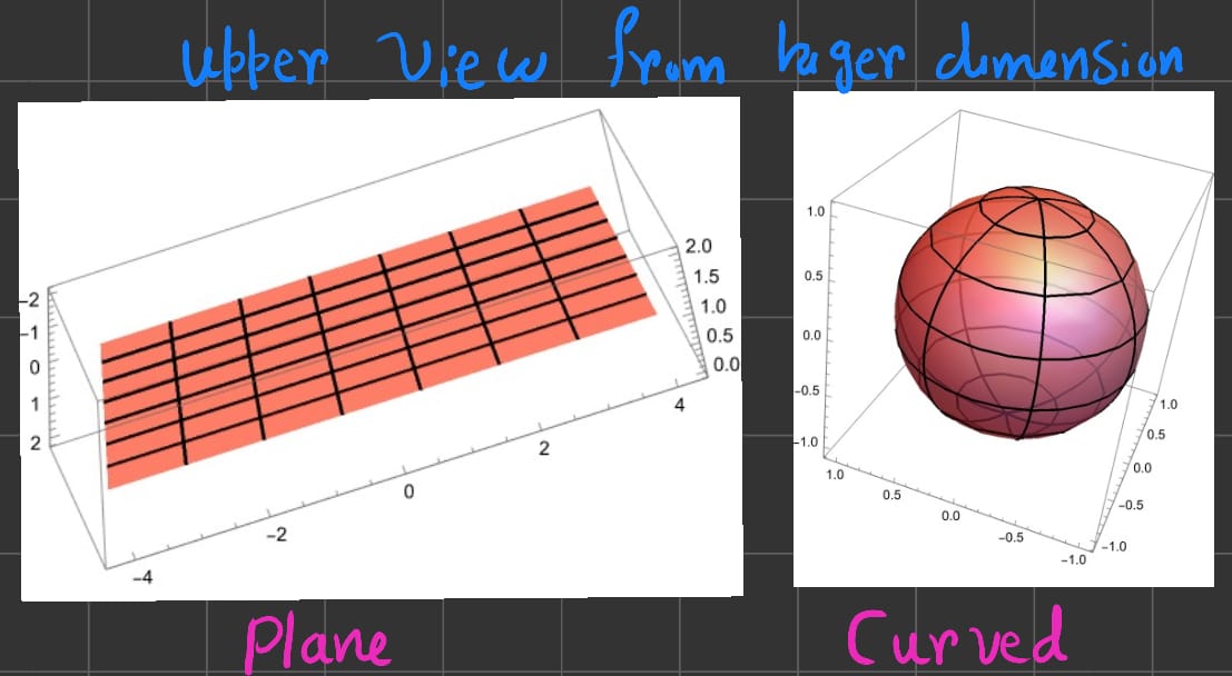
It all starts with a very simple question, How can we tell if a space is curved or flat?
Well, It seems very simple right?, just by looking at the surface.
.
So, to use this method, if we have a \(n-D\) surface, then we need to use \((n+1) -D\) space. But most time we don't have a luxory of doing this nor we have a image of the surface in higher dimension.
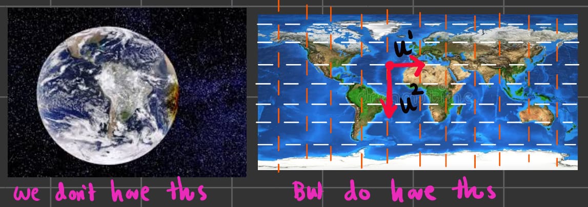
As an example, earth is spherical but we live on it. So, we only have maps but no picture of the surface(until we have spacecrafts).
.
This exact thing is done by Riemann Curvature Tensor. The whole idea is based upon the idea of Parallel Transport of vectors.
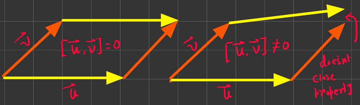
To define Riemann Curvature Tensor, we need to define two vector fields let's say \(\vec{U}\) and \(\vec{V}\) with the assumption that \([\vec{U}, \vec{V}]=0\). Using this two vectors we form a parallelogram as shown.
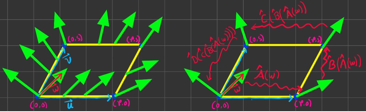
\(\hat{A}\) takes in \(\vec{W}\) and maps it to parallel transport of \(\vec{W}\) at \((r,0)\).
\(\hat{B}\) takes in transported \(\vec{W}\) from \((r,0)\) and maps it to parallel transport of \(\vec{W}\) at \((r,s)\).
\(\hat{C}\) takes in transported \(\vec{W}\) from \((r,s)\) and maps it to parallel transport of \(\vec{W}\) at \((0,s)\).
Finally, \(\hat{D}\) takes it back to it's initial position.
If the space is curved, we know after the parallel transport the vector will be different. The change in the vector can be written as \(\vec{W} - \hat{D}\hat{C}\hat{B}\hat{A}\vec{W}\).
From, here we define the Riemann Curvature Tensor(\(R\)) as,
\[ R(\vec{U},\vec{V})\vec{W} = \lim_{r,s\to 0} \frac{\vec{W} - \hat{D}\hat{C}\hat{B}\hat{A}\vec{W}}{rs} \]A little simplification gives us,
\[ R(\vec{U},\vec{V})\vec{W} = \nabla_{\vec{U}}\nabla_{\vec{V}}\vec{W} - \nabla_{\vec{V}}\nabla_{\vec{U}}\vec{W} - \nabla_{[\vec{U},\vec{V}]}\vec{W} \]where \(\nabla\) represent covariant derivative.
In component form, the formula of this tensor becomes,
\[ R^{\alpha}_{\beta \mu \nu} = \partial_\mu \Gamma^{\alpha}_{\nu \beta} - \partial_\nu \Gamma^{\alpha}_{\mu \beta} + \Gamma^{\alpha}_{\mu \lambda}\Gamma^{\lambda}_{\nu \beta} - \Gamma^{\alpha}_{\nu \lambda}\Gamma^{\lambda}_{\mu \beta} \]This is very big and really very hard to remember. Our main goal is to find a way to remember this (I hate this but it really helps).
Mnemonic for the Tensor
To start this, let's represent \(\partial_{\fbox{}}\) as \(P\) and for the Christoffel Symbols \(\Gamma^{\fbox{}}_{\fbox{}\fbox{}}\) as \(C\). Here \(\fbox{}\) is like a placeholder for \(\alpha\), \(\beta\), \(\mu\) and \(\nu\). So, we can write the pattern as,
\[ R^{\alpha}_{\beta \mu \nu} = + P\cdot C - P \cdot C + C \cdot C - C \cdot C \]So, first point to remember: Write two \(PC\) and \(CC\) with alternating signs, starting with \(+\). So, we have,
\[ R^{\alpha}_{\beta \mu \nu} = + \partial_{\fbox{}}\Gamma^{\fbox{}}_{\fbox{}\fbox{}} - \partial_{\fbox{}}\Gamma^{\fbox{}}_{\fbox{}\fbox{}} + \Gamma^{\fbox{}}_{\fbox{}\fbox{}} \Gamma^{\fbox{}}_{\fbox{}\fbox{}} - \Gamma^{\fbox{}}_{\fbox{}\fbox{}} \Gamma^{\fbox{}}_{\fbox{}\fbox{}} \]Now, for \(\alpha\) put that in the correct places. This is obvious.
\[ R^{\alpha}_{\beta \mu \nu} = + \partial_{\fbox{}}\Gamma^{\alpha}_{\fbox{}\fbox{}} - \partial_{\fbox{}}\Gamma^{\alpha}_{\fbox{}\fbox{}} + \Gamma^{\alpha}_{\fbox{}\fbox{}} \Gamma^{\fbox{}}_{\fbox{}\fbox{}} - \Gamma^{\alpha}_{\fbox{}\fbox{}} \Gamma^{\fbox{}}_{\fbox{}\fbox{}} \]After this, for the \(CC\) terms, put same index in the cross placeholders as shown (in red colour),
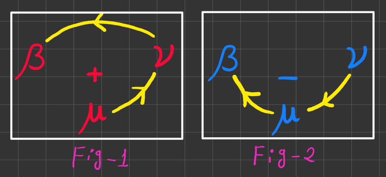
\[ R^{\alpha}_{\beta \mu \nu} = + \partial_{\fbox{}}\Gamma^{\alpha}_{\fbox{}\fbox{}} - \partial_{\fbox{}}\Gamma^{\alpha}_{\fbox{}\fbox{}} + \Gamma^{\alpha}_{\fbox{}\textcolor{lime}{\lambda}} \Gamma^{\textcolor{lime}{\lambda}}_{\fbox{}\fbox{}} - \Gamma^{\alpha}_{\fbox{}\textcolor{lime}{\lambda}} \Gamma^{\textcolor{lime}{\lambda}}_{\fbox{}\fbox{}} \]The next step is to take our \(3\) index \(\beta\), \(\mu\) and \(\nu\) & push the middle(\(m\)) one down as shown.

.
Now, for the positive(\(+\)) terms, we start from \(\mu\) and go anticlockwise direction & for the negative(\(-\)) terms, we start from \(\nu\) and go clockwise term, as we do for angle measurment.
The picture below should show what I mean.
.
Reproducing our result.
Hope this helps you in some way. If you like it then share with others if possible.
If you have some queries, do let me know in the comments or contact me using my using the informations that are given on the page About Me.