
Introduction to Monte Carlo Integration
Hi again!
So, once again you are here... good good!...
Monte Carlo Method,a statistical method of understanding complex physical or mathematical systems by using randomly generated numbers as input into those systems to generate a range of solutions. The likelihood of a particular solution can be found by dividing the number of times that solution was generated by the total number of trials. By using larger and larger number of trials, the likelihood of getting solutions can be determined more accurately.
We can say Monte Carlo Integration Method is a way to get order from randomness.
Introduction
Monte Carlo Integration is a technique for numerical integration using random numbers. It is a particular Monte Carlo method that numerically computes a definite integral.
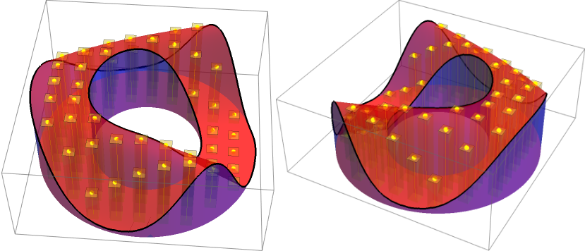
Rectangular Boxes under the Surface with randomly chosen position. We will try to understand what this means in this blog.
Well due to the random sampling, you may think it is not very efficient and for 1D it is quite true. But this one truly shines in it's extension to higher dimensions. In our current world from Image Processing, Ray Tracing to studying the nature of fundamental particles, all of these needs higher dimensional integrations. Hence, this method is really important.
Based on the law of probability everything is possible because the sheer existence of possibility confirms the existence of impossibility.
The Monte Carlo method is used in a wide range of subjects, including mathematics, physics, biology, engineering and finance, and in problems in which determining an analytic solution would be too time-consuming.
Our goal in this blog will be to understand basic Monte Carlo Integration method for a single variable function.
Before understanding the Monte Carlo Integration, we need to review few statistical ideas. So, let's see those for the sake of everyone.
Recap of some Statistical Ideas
I will keep it as brief as possible.
Let's start with the idea of Expected Value. We can think of expected value as the weighted average of a process.
What do I mean by this?
First let's see for the case of discrete variables. Suppose we have 14 people in a room.
| Age(year) | People with age(\(N(age)\)) |
|---|---|
| 14 | 1 |
| 15 | 1 |
| 16 | 3 |
| 22 | 2 |
| 24 | 2 |
| 25 | 5 |
So here \(N(14) = 1\), \(N(15) = 1\), \(N(16) = 3\), \(N(22) = 2\), \(N(24) = 2\) and \(N(25) = 5\). So, any number(age) which is not there like \(17\), \(N(17) = 0\).
\[ \sum_{j=0}^{\infty}N(j) = N = 14 \]Let's find the corresponding probabilities.
| \(N(age)\) | Probability(\(P(j) = \frac{N(j)}{N}\)) |
|---|---|
| \(N(14)=1\) | \(P(14)=\frac{1}{14}\) |
| \(N(15)=1\) | \(P(15)=\frac{1}{14}\) |
| \(N(16)=3\) | \(P(16)=\frac{3}{14}\) |
| \(N(22)=2\) | \(P(22)=\frac{2}{14}\) |
| \(N(24)=2\) | \(P(24)=\frac{2}{14}\) |
| \(N(25)=5\) | \(P(25)=\frac{5}{14}\) |
Another interesting thing here is,
\[ \sum_{j=0}^{\infty}P(j) = 1 \]Here few points should be noted:
The most probable age is \(25\) as five people share that age.
The average or mean age is \((14+15+3\times 16 + 2 \times 22 + 2\times 24 + 5\times 25)/14 = 21\). The age \(21\) is not even present in the group of people.
This is the normal average with each element having equal weight of 1. But in most cases doing this doesn't provide too many information. Like we clearly know that people of age \(25\) contribute the most. So, adding this type of information, we introduce weighted average, i.e., Expected Value . It is defined as,
\[ \langle j \rangle = \frac{\sum_{0}^{\infty} j N(j)}{N} = \sum_{0}^{\infty} j \frac{N(j)}{N} = \sum_{0}^{\infty} j P(j) \]Notice, the weight is just the probability of \(j\) as probability informs which values contribute the most.
So,
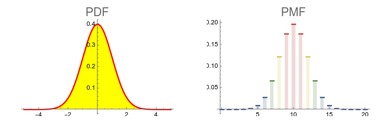
\[ \langle f(x) \rangle = \sum_{i = 0}^{\infty} f(x_i) P(x_i) \]So, for any function \(f(x)\) the expected value can be given by eqn-(4). Here \(P(x_i)\) tells us the probability of the function to have the value \(f(x_i)\). Sometimes this \(P(x)\) is called PMF(Probability Mass Function).
In case of our example of \(PMF\) takes discrete values(\(f(x)\) also takes discrete values, some fixed value of \(x_i\) are only present). But what if our variable is continious?
Well, then the equation for expectation value/expected value is written as,
\[ \langle f(x) \rangle = \int_{-\infty}^{\infty}dx f(x) p(x) \]Here \(p(x)\) is called PDF,i.e., Probability Density Function. The reason for calling it PDF is that \(p(x)dx\) represents the probability of getting the value of the function f(x) in the range of \(x\) and \(x+dx\).
The probability of \(f(x)\)'s value to be in between \(f(a)\) to \(f(b)\) is given by,
\[ P(a\leq x \leq b) = \int_{a}^{b}dx\ p(x)\]\(p(x)\) must satsify,
\(p(x)\geq 0\), for all \(x\in \mathbb{R}\).
\(p\) is piecewise continious.
It also satisfies \(\int_{-\infty}^{\infty}dx p(x) = 1\).
Note that the PDF is continuous and PMF is discontinious.
Another important quantity in this topic is Cumulative Distribution Function(CDF).
This is defined as (in continious case),
For discrete variables, it is
\[ F(x_i) = \sum_{j=0}^{j=i}P(x_j) \]I hope you have understood the concepts upto this point. Two formulas of expected value is,
\(\langle c f(x_i) \rangle = c \langle f(x_i) \rangle\)
\(\langle \sum_i f(x_i) \rangle = \sum_i \langle f(x_i) \rangle\)
Another important idea is Variance. Intuitively, Variance tells us the spread of our data, i.e., how much random variable \(X\) is expected to differ from it's expected value. Mathematically, It is given by,
\[ Var(X) = \langle (X - \langle X \rangle )^2 \rangle = \langle X^2 \rangle - \langle X \rangle ^2 \]If for any random variable \(X\), the variance is big, this means the values which \(X\) randomly takes are very different from the expected value of \(X\).
In the same way, if the variance is small, then it means \(X\) takes values randomly which are very close to \(\langle X \rangle\).
Two properties of variances which we will need are,
\(Var(cX) = c^2 Var(X)\) for any constant \(c\).
\(Var(\sum_i X_i) = \sum_i Var(X_i)\)
I think it's becoming lengthy... So, let's stop here and dive straight into the integrations.
Monte Carlo Integration
Let's take an example to understand the method. Suppose we want to find the integration of the function \(g(x) = \sqrt{1-x^2}\) in the range \([-1,1]\),i.e., we want to compute,
\[ I = \int_{-1}^{1}dx\ \sqrt{1-x^2} \]Note: Visually, this is the area of a semi-circle of radius 1.
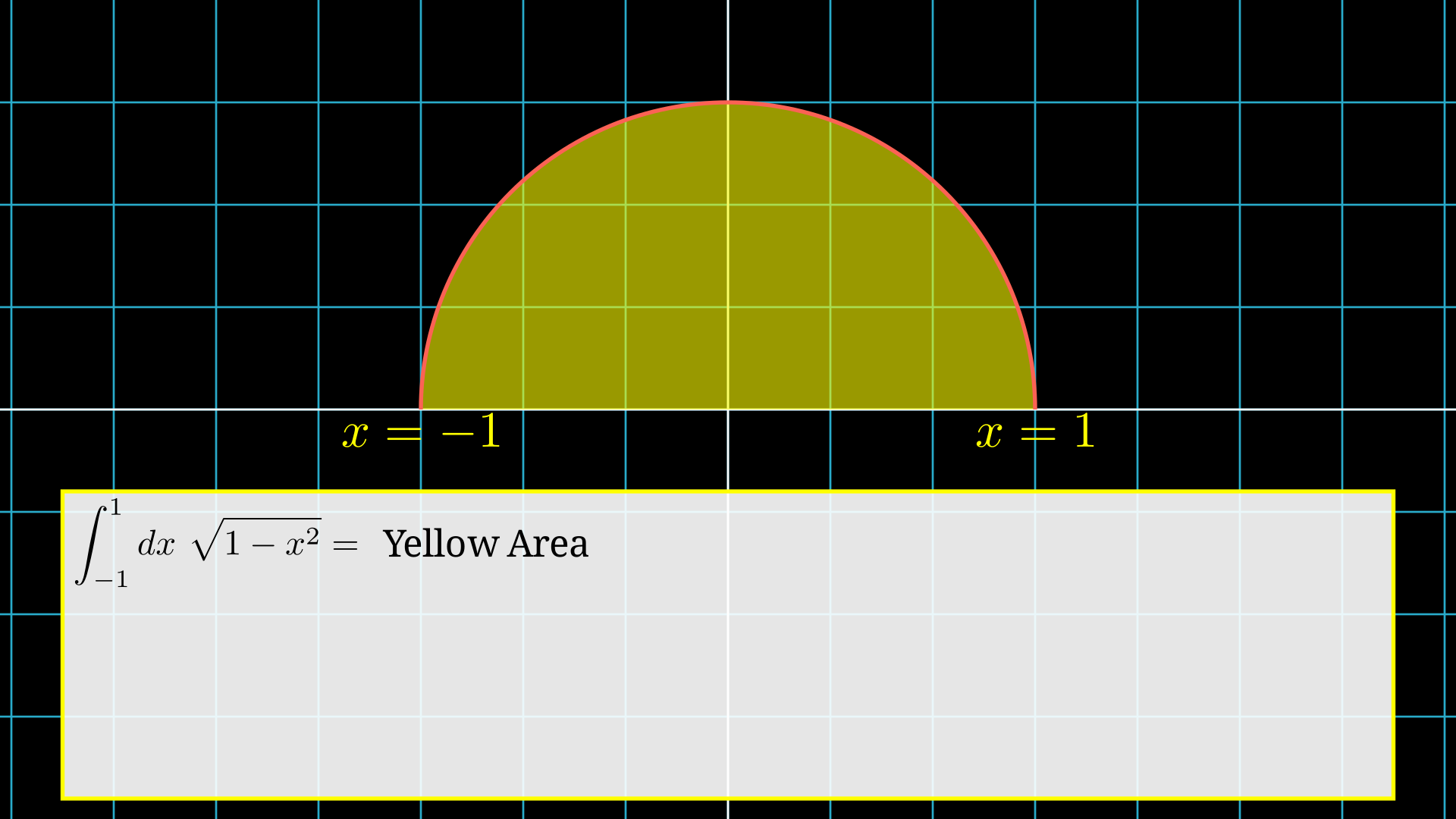
Integration is equals to the area under the curve, i.e., yellow region area.
Monte Carlo Method is very simple. The steps are as following:
Uniformly sample the region \(-1\leq x \leq 1\), i.e., let's say we choose \(N= 100\) random values from \(-1\) to \(1\). The samples really doesn't have to be uniform (will discuss elaborately in other blog).
For each random x value, we evaluate the function at that point and assume the function is constant throughout the interval. \(N\) has to be quite large to get a good estimate.
Finally take the average of all the f values multiplied by the interval length.
To understand these three steps, watch the animation below.
First we choose a point randomly in the interval.
Then we find corresponding \(f(x)\).
After that we find the area of the rectangle which is \(f(x)\times(b-a)\) (Here \(b=1\) and \(a= -1\)).
Finally we repeat it \(N=4\) times and then take the average.
So, for any function \(f(x)\), if we want to find,
\[ I = \int_a^b dx\ f(x) \]Then using Monte Carlo Integration method, we have,
where \(x_i\) is some random number in between \(x=a\) and \(x=b\). \(N\) is the number of samples we want.
Let's see the proof.
Proof and Estimate
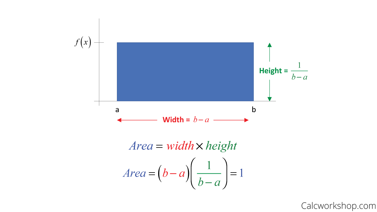
The proof is pretty easy. We will use uniform PDF for that. In the region \(x=a\) to \(x=b\), we want a uniform PDF. Hence, the value should be
\[p(x) = \frac{1}{(b-a)}\]for \(a\leq x \leq b\), else \(p(x)=0\). This is the case we consider as \(\int_{a}^{b}dx\ p(x) = 1\) (see the Figure below).
Let's find it's expected value.
\[ \langle E_N \rangle = \langle \frac{b-a}{N}\sum_{i=1}^N f(x_i) \rangle = \frac{b-a}{N}\sum_{i=1}^N \langle f(x_i) \rangle = \frac{b-a}{N}\sum_{i=1}^N\int_a^b dx\ f(x) p(x) \]So, finally
\[ \langle E_N \rangle = \frac{1}{N}\sum_{i=1}^N\int_a^b dx\ f(x) = \int_a^b dx \ f(x) \]Hence, we conclude the proof. But a question may arise, is it true only for uniform distribution? or it is true for any distribution?
The answer is: Any distribution. It's also very easy to prove (See any book on the topic, you will find it).
But is this method good? To answer this we compute it's Variance. Let's do so,
\[ Var(E_N) = Var\Bigg( \frac{1}{N}\sum_{i=1}^N \frac{f(x_i)}{p(x_i)}\Bigg) = \frac{1}{N} \sum_{i=1}^N Var\Bigg( \frac{f(x)}{p(x)}\Bigg) \]Here we have assumed each sample are independent of each other. So, we have,
\[ Var(E_N)\propto \frac{1}{N} \to Error \propto \frac{1}{\sqrt{N}} \]This implies Increasing the N, i.e.,by increasing sample number the error of our method will decrease.
But it also tells us going from 10 samples to 100 samples will reduce the error more, than if we go from 10,000 to 1,00,000.
For a beautiful introduction to Monte Carlo method watch this video by Prof.John Guttag
Simulating Monte-Carlo Integration.
Let's use all that we have just learnt in julia language.
We will be using the semi-circle integral. Let's study all the lines one by one. For example we will use Distributions package for using PDF.
First import the library.
julia> using DistributionsNow let's define the function \(f(x) = \sqrt{1-x^2}\).
julia> f(x) = sqrt(1-x^2)Define \(N\), \(a\) and \(b\).
julia> N = 1000; a = -1; b = 1;Sample \(N\) values uniformly in between \(a\) and \(b\).
julia> x_v = rand(Uniform(a,b),N)Finally, the integration value will be calculated by.
julia> Inte = (b-a)/N * sum(f.(x_v))I hope, you have understood this idea. Now, let's write a function to do the whole job and get some result.
using Distributions

function Inte_monte1D(f,N,a,b)
    x_v = rand(Uniform(a,b),N)
    return ((b-a)/N)*sum(f.(x_v))
end
g(x) = sqrt(1 - x^2)
N = 1000; a = -1; b = 1;
vv = Inte_monte1D(g,N,a,b)
println("The area of semi-circle for N = $N , a = $a and b = $b is ",vv)
The output is:
The area of semi-circle for N = 1000 , a = -1 and b = 1 is 1.5817145092207434
Now, let's calculate the integration for different \(N\) values and calculate the error in each case.
using Distributions, DataFrames

function Inte_monte1D(f,N,a,b)
    x_v = rand(Uniform(a,b),N)
    return ((b-a)/N)*sum(f.(x_v))
end

inte_results = Float64[]
error = Float64[]
N_vals = Int64[]
a = -1; b = 1;
g(x) = sqrt(1-x^2)
for i in 1:8
    vv = Inte_monte1D(g,10^i,-1,1)
    actual_val = pi/2
    append!(inte_results,vv)
    append!(error,abs(actual_val-vv))
    append!(N_vals,10^i)
end

df = DataFrame(N = N_vals, Integration_Result = inte_results, Error = error)
print(df)
The output is:
8×3 DataFrame
 Row │ N          Integration_Result  Error
     │ Int64      Float64             Float64
─────┼────────────────────────────────────────────
   1 │        10             1.71039  0.139592
   2 │       100             1.58069  0.00989215
   3 │      1000             1.55854  0.0122612
   4 │     10000             1.57659  0.00579797
   5 │    100000             1.57121  0.000415458
   6 │   1000000             1.57111  0.00031825
   7 │  10000000             1.57059  0.000207658
8 │ 100000000 1.57078 1.46366e-5We can make the code much faster (although it is already very fast) using parallel computing and many more modern blackmagic of different algorithms & technology. But we will not discuss those here but a little example doesn't hurt.
using Distributions
function Inte_monte1D_thread(f,N,a,b,th_num=Threads.nthreads())
tempo = zeros(Float64, th_num)
n = Int(floor(N/th_num))
Threads.@threads for i in eachindex(tempo)
xv = rand(Uniform(a,b),n)
tempo[Threads.threadid()] += sum(f.(xv))
end
return ((b-a)/N)*sum(tempo)
end
function Inte_monte1D(f,N,a,b)
xv = rand(Uniform(a,b),N)
return ((b-a)/N)*sum(f.(xv))
end
a = -1; b = 1;
h(x) = sqrt(1-x^2)
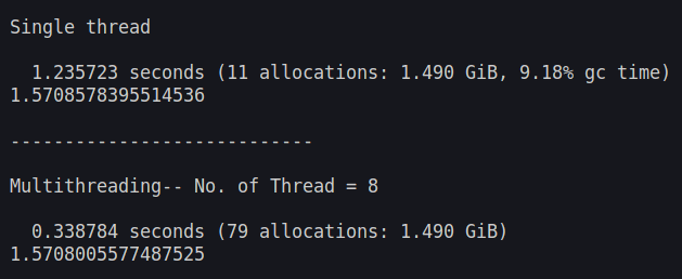
N =10^8
println("Single thread")
@time Inte_monte1D(h,N,-1,1)
pi/2
println("----------------------------")
println("Multithreading-- No. of Thread = ",Threads.nthreads())
@time Inte_monte1D_thread(h,N,-1,1)The output is:
As we go to higher dimensions, the Monte Carlo method truly shines. It is free from the curse of dimensionality.
I hope you all get to know something new or maybe it was like a refreshment to your old memories.
If you have some queries, do let me know in the comments or contact me using my using the informations that are given on the page About Me.