- What we demand of a shape descriptor
- Hadwiger's theorem: in \(d\) dimensions there are exactly \(d+1\)
- A short primer on curvature
- The Minkowski sum and the first definition of the functionals
- The Euler characteristic, concretely
- From a fixed body to a random field: flood the landscape
- The Gaussian baseline and its Hermite structure
- Measuring the functionals on a pixel grid
- The fit: measure all four functionals and overlay the theory
- Why this matters: what the power spectrum cannot see
- Non-Gaussianity: how the curves shift
- A real application: is a dust-cleaned sky Gaussian?
- The CMB as a worked example
- The whole story in eight lines
Minkowski Functionals: Measuring the Shape of the Universe
How do you put a number on the shape of a thing? Not where it is or how it is turned, but its actual form: how big, how frilly its edge, how it bends, how many holes. This is a self-contained tour from that everyday question all the way to how cosmologists use the answer to test whether the early Universe was Gaussian.
Hi again!
Suppose I hand you a map (the temperature of the sky, a slab of the cosmic density field, a grayscale photo, anything) and ask you to describe its shape to someone who can't see it. You'd probably say things like:
"It is big": a statement about content (area or volume).
"Its edge is long and ragged": about the boundary.
"It bulges here and pinches there": about curvature.
"It's three blobs, one with a hole through it": about topology (connectivity).
That list turns out to be essentially complete. Content, boundary, curvature, and connectivity are not an arbitrary grab-bag. They are the Minkowski functionals of a body, and a 1957 theorem of Hadwiger says there are no others. This post builds them from scratch, derives their exact values for a Gaussian random field, checks every step with a computer-algebra system and simulations, and then shows why this is one of cosmology's sharpest tools.
The power spectrum tells you how loud each note is. Minkowski functionals tell you the shape of the song, and a Gaussian universe can only sing in a handful of closed-form curves.What we demand of a shape descriptor
Let \(K\) be a "body": a compact, reasonably smooth chunk of space, like a filled ball, a cube, or the patch of sky where the temperature exceeds some value. A functional \(F\) assigns one real number \(F(K)\) to each such body. We'll only call \(F\) a legitimate morphological descriptor if it obeys three axioms:
(M1) Motion invariance. \(F(gK)=F(K)\) for any rotation+translation \(g\). The intrinsic shape of a coffee mug can't depend on whether it's on the table or in your hand. This is the coordinate-free demand, and it is what separates what the object is from where it is.
(M2) Additivity. \(F(A\cup B)=F(A)+F(B)-F(A\cap B)\). Careful counting: assemble a region from overlapping pieces and you subtract the double-counted overlap. Additivity is also what makes these statistics locally computable. You can scan a pixelated map cell by cell and accumulate, correcting for shared edges, instead of holding the whole dataset at once.
(M3) Continuity. Wiggle the boundary a little, the number changes a little. This rules out pathological descriptors that jump, and makes the functionals robust to noise and finite pixelisation.
It's worth noticing how much these axioms exclude. The raw count of pixels above a threshold jumps by \(\pm1\) under an infinitesimal change, so it fails (M3). A statistic that depends on the orientation of your coordinate axes fails (M1). The fractal dimension of a coastline isn't additive, so it fails (M2). Minkowski functionals are the descriptors that pass all three at once.
Hadwiger's theorem: in \(d\) dimensions there are exactly \(d+1\)
Here is the structural fact at the heart of the subject.
Hadwiger's characterisation theorem (1957). In \(\mathbb R^d\), every functional satisfying (M1)-(M3) is a linear combination of exactly \(d+1\) fundamental ones \(W_0,W_1,\dots,W_d\) (the Minkowski functionals, also called quermassintegrals): \(\;F(K)=\sum_{\nu=0}^{d} c_\nu\, W_\nu(K).\)
So if you ever invent a clever new coordinate-free, additive, continuous shape statistic, Hadwiger guarantees you have discovered nothing new. Your statistic is secretly a weighted sum of the same \(d+1\) numbers. For a concrete taste: in 2D, the "isoperimetric ratio" perimeter\(^2\)/area looks like a brand-new shape number, but perimeter is just \(4W_1\) and area is \(W_0\), so the ratio is \(16W_1^2/W_0\), a combination of two functionals you already had. Compare this with \(n\)-point correlation functions, which form an infinite tower. The MFs are a finite, complete alternative at the level of additive morphology. In the dimensions that matter to physics:
| Dimension \(d\) | No. of MFs | What they measure |
|---|---|---|
| \(d=1\) (a line) | 2 | length, endpoint count (\(\chi\)) |
| \(d=2\) (a sky map) | 3 | area, perimeter, Euler characteristic (\(\chi\)) |
| \(d=3\) (a volume) | 4 | volume, surface area, integrated mean curvature, \(\chi\) |
Two of the higher functionals are integrals of curvature, so we need to build that idea honestly first.
A short primer on curvature
Curvature of a curve. Walk a curve at unit speed; your heading (the unit tangent) rotates as you go. The rate of that rotation is the curvature \(\kappa\). A straight line has \(\kappa=0\); a circle of radius \(R\) turns at constant rate \(\kappa=1/R\). A tight circle has large \(\kappa\), a vast one is nearly straight, and \(R=1/\kappa\) is the radius of curvature.
Curvature of a surface. At a point \(P\), stand a knife-blade along the surface normal and slice; the cut is a plane curve with some curvature. Rotate the blade around the normal and the curvature changes. The largest and smallest values are the two principal curvatures \(\kappa_1=1/R_1\) and \(\kappa_2=1/R_2\). From them we build two combinations:
\[ H=\tfrac12(\kappa_1+\kappa_2)\quad\text{(mean curvature)}, \qquad K_G=\kappa_1\kappa_2\quad\text{(Gaussian curvature)}. \]Mean curvature \(H\) answers "which way, and how strongly, does it bend on average?" It separates outward lumps (\(H>0\)) from inward necks (\(H<0\)). Gaussian curvature \(K_G\) answers "what kind of point is this?":
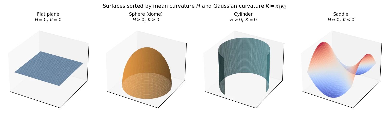
A flat plane (both curvatures zero), a sphere (both positive), a cylinder (one direction flat, K=0), and a saddle (opposite signs, K<0). Gauss's Theorema Egregium says K is intrinsic: an ant living on the surface could measure it from internal distances alone, with no reference to the surrounding 3D space.
Gauss-Bonnet: curvature encodes topology. The deepest fact about Gaussian curvature is that its integral over a surface is locked to a topological integer. For a surface \(\Sigma\) with boundary \(\partial\Sigma\),
\[ \int_\Sigma K_G\,dA \;+\; \int_{\partial\Sigma}\kappa_g\,ds \;+\; \sum_i \theta_i \;=\; 2\pi\,\chi(\Sigma), \]where \(\kappa_g\) is the geodesic curvature of the boundary (how it bends within the surface), the \(\theta_i\) are exterior angles at corners, and \(\chi\) is the Euler characteristic. For a closed surface this reduces to \(\frac{1}{2\pi}\int K_G\,dA=\chi\): a sphere has \(\chi=2\), a torus has \(\chi=0\), and each extra handle lowers \(\chi\) by 2. You can push curvature around the surface all you like and the integral never budges. This is the bridge from a local, smooth quantity (curvature) to a global, integer one (topology), and it is exactly why one Minkowski functional is a pure connectivity counter.
The Minkowski sum and the first definition of the functionals
There are two equivalent ways to define the functionals. The first is wonderfully physical: inflate the body and watch how its volume grows. To make that precise we need the Minkowski sum.
Minkowski sum. For two sets \(A,B\), define \(A\oplus B=\{\mathbf a+\mathbf b:\mathbf a\in A,\ \mathbf b\in B\}\).
Two pictures, same operation: stamping (drop a copy of \(B\) at every point of \(A\) and union them) and sweeping (slide \(B\)'s reference point over all of \(A\); the swept region is \(A\oplus B\)). When \(B=\varepsilon B_1\) is a ball of radius \(\varepsilon\), the sum \(A\oplus\varepsilon B_1\) is exactly all points within distance \(\varepsilon\) of \(A\), a uniform fattening. As a concrete case, a \(2\times2\) square fattened by a disc of radius \(\varepsilon\) becomes the square plus a rim: four flat strips of area \(2\cdot(4\varepsilon)\) down the sides and four quarter-discs at the corners that assemble into one full disc \(\pi\varepsilon^2\). (If you've met morphological dilation in image processing, or configuration-space obstacles in robot path-planning, you've already used this.)
Definition I: the Steiner inflation formula
Take a convex body \(K\), inflate it to its parallel body \(K\oplus\varepsilon B\), and measure the new volume. Steiner showed in 1840 that this is a polynomial in \(\varepsilon\):
\[ \mathrm{Vol}(K\oplus\varepsilon B)=\sum_{\nu=0}^{d}\binom{d}{\nu}W_\nu(K)\,\varepsilon^{\nu}. \]The coefficients \(W_\nu\) are (up to the binomials) the Minkowski functionals. Why does inflation sort geometry by powers of \(\varepsilon\)? Because the new material arrives in geometrically distinct layers:
the \(\varepsilon^0\) term is the original body, its content (volume or area);
the \(\varepsilon^1\) layer is a uniform slab over the boundary, its volume proportional to the surface area;
higher powers fill the rounded edges and corners, set by how the boundary curves, with the top power packaging up the topology.
The Steiner polynomial literally sorts a body's geometry by how strongly each feature responds to inflation. Reading off the coefficients hands you the functionals one by one. Watch it on a square:

Inflating a square by ε. The added area splits into four flat slabs (orange, proportional to perimeter, the ε¹ term) and four corner quarter-discs that assemble into one full disc (green, πε², the ε² term, carrying the Euler characteristic χ=1). Each power of ε isolates one functional.
In formulas, a square of side \(a\) has \(\text{Area}=\underbrace{a^2}_{\varepsilon^0}+\underbrace{4a}_{\varepsilon^1}\varepsilon+\underbrace{\pi}_{\varepsilon^2}\varepsilon^2\), giving \(W_0=a^2\) (area), \(W_1=2a=\tfrac12(\text{perimeter})\), and \(W_2=\pi=\pi\chi\) with \(\chi=1\). Put numbers on it: for \(a=2\) and \(\varepsilon=0.5\), the inflated area is \(4+8(0.5)+\pi(0.25)=8.785\), and reading off the powers of \(\varepsilon\) recovers the original area \(4\), the half-perimeter \(4\), and the constant \(\pi\) that holds the topology. The same exercise on a 3D ball of radius \(R\) gives \(\mathrm{Vol}=\tfrac43\pi(R+\varepsilon)^3\), whose four coefficients are \(W_0=\tfrac43\pi R^3\) (volume), \(W_1=\tfrac43\pi R^2\) (one third the surface), \(W_2=\tfrac49\pi R\), and \(W_3=\tfrac49\pi\), which is independent of \(R\), the hallmark of a topological quantity (\(\chi=1\) for any convex body).
Definition II: the curvature-integral form
The same coefficients can be written as surface integrals over \(\partial K\), where the physical meaning is most vivid. Using the normalisation standard in cosmology (Schmalzing & Buchert 1997), in 3D:
\[ \begin{aligned} V_0 &= \int_K d^3x &&\text{volume}\\ V_1 &= \tfrac16\!\int_{\partial K}\! dS &&\propto\ \text{surface area}\\ V_2 &= \tfrac1{6\pi}\!\int_{\partial K}\! H\,dS &&\propto\ \text{integrated mean curvature}\\ V_3 &= \tfrac1{4\pi}\!\int_{\partial K}\! \tfrac{dS}{R_1R_2} &&=\ \text{Euler characteristic } \chi \end{aligned} \]In 2D, for a region \(Q\) with boundary curve \(\partial Q\):
\[ V_0=\int_Q da,\qquad V_1=\tfrac14\!\int_{\partial Q}\! d\ell,\qquad V_2=\tfrac1{2\pi}\!\int_{\partial Q}\!\kappa\,d\ell=\chi. \]In plain words, in 2D: \(V_0\) is what fraction of the map is covered; \(V_1\) is the contour length (a smooth disc has the least perimeter for its area, a crinkled boundary far more, so it measures coastline complexity); and \(V_2\) is the Euler characteristic, \(\chi=\#(\text{isolated spots})-\#(\text{holes})\). The funny prefactors (\(\tfrac14\), \(\tfrac1{2\pi}\), and so on) are the conventional Hadwiger normalisation. As a sanity check, the 2D disc of radius \(R\) gives \(V_0=\pi R^2\), \(V_1=\tfrac14(2\pi R)=\tfrac{\pi R}{2}\), and \(V_2=\tfrac1{2\pi}\cdot\tfrac1R\cdot2\pi R=1=\chi\). The topological functional is blind to shape: \(V_2=1\) for any simply-connected 2D region, whether disc, square, triangle, or blob.
The Euler characteristic, concretely
Because \(V_2\) (2D) and \(V_3\) (3D) are purely topological, they deserve a careful picture. They are what distinguishes a meatball from a sponge:

Count pieces, subtract holes. Left (meatball): 5 isolated clumps, no holes, so χ = +5. Right (sponge): one connected body riddled with 5 holes, so χ = 1−5 = −4. Two fields can have the same power spectrum and opposite topology; only χ can tell them apart.
The quickest way to build intuition is to read printed letters as 2D shapes. A solid blob, the letter "L", or the letter "C" each is one piece with no hole, so \(\chi=1\). The letters "O", "A", "D", and the digit "0" are one piece with one hole, so \(\chi=1-1=0\). The letter "B" and the digit "8" are one piece with two holes, so \(\chi=1-2=-1\). The word "OXO" is three separate pieces, two with a hole, so \(\chi=3-2=1\). You are just counting components and subtracting holes.
More formally, \(\chi=\sum_k(-1)^k\beta_k\) in terms of the Betti numbers: \(\beta_0\) counts connected components, \(\beta_1\) counts independent loops or tunnels, and \(\beta_2\) counts enclosed cavities. Morse theory ties \(\chi\) to the critical points of the field: in 2D each maximum contributes \(+1\), each saddle \(-1\), and each minimum \(+1\). Sweeping a threshold means watching critical points enter and leave the region, and \(\chi(\nu)\) records every topological event along the way. That last idea is the bridge to cosmology.
From a fixed body to a random field: flood the landscape
Everything so far described one fixed body. The bridge to cosmology is a single idea: turn a continuous field into a family of bodies by thresholding it.
Read your map as a landscape, with the value \(u(\mathbf x)\) as an altitude. Pick a number \(\nu\), a water level, and flood the world to that height. Everything above water is the excursion set
\[ Q_\nu=\{\mathbf x : u(\mathbf x)\ge\nu\}, \]and the coastline is the level set \(\partial Q_\nu=\{u=\nu\}\).

Left: along a 1D slice the field crosses ν four times, so Qν is two intervals and ∂Qν is four points. Right: in 2D, Qν is the orange land where u>ν and ∂Qν is the red coastline. The three functionals measure its area (V₀), boundary length (V₁), and integrated geodesic curvature (V₂).
At each water level we photograph the dry land and measure its \(d+1\) Minkowski functionals; sweeping \(\nu\) from \(+\infty\) down to \(-\infty\) turns each functional into a curve \(V_k(\nu)\). Drag the slider and watch the land, the coastline, and all three functionals move together:
Drag the slider. Top: the terrain with the blue water plane. Bottom-left: the top-down excursion set Qν with orange land, blue sea, red coastline ∂Qν: watch islands appear, merge into one lacy continent, then drown leaving isolated lakes. Bottom-right: the three functionals vs ν with a marker at the current level.
As the slider sweeps you pass through three regimes, and they drive the shape of every MF curve:
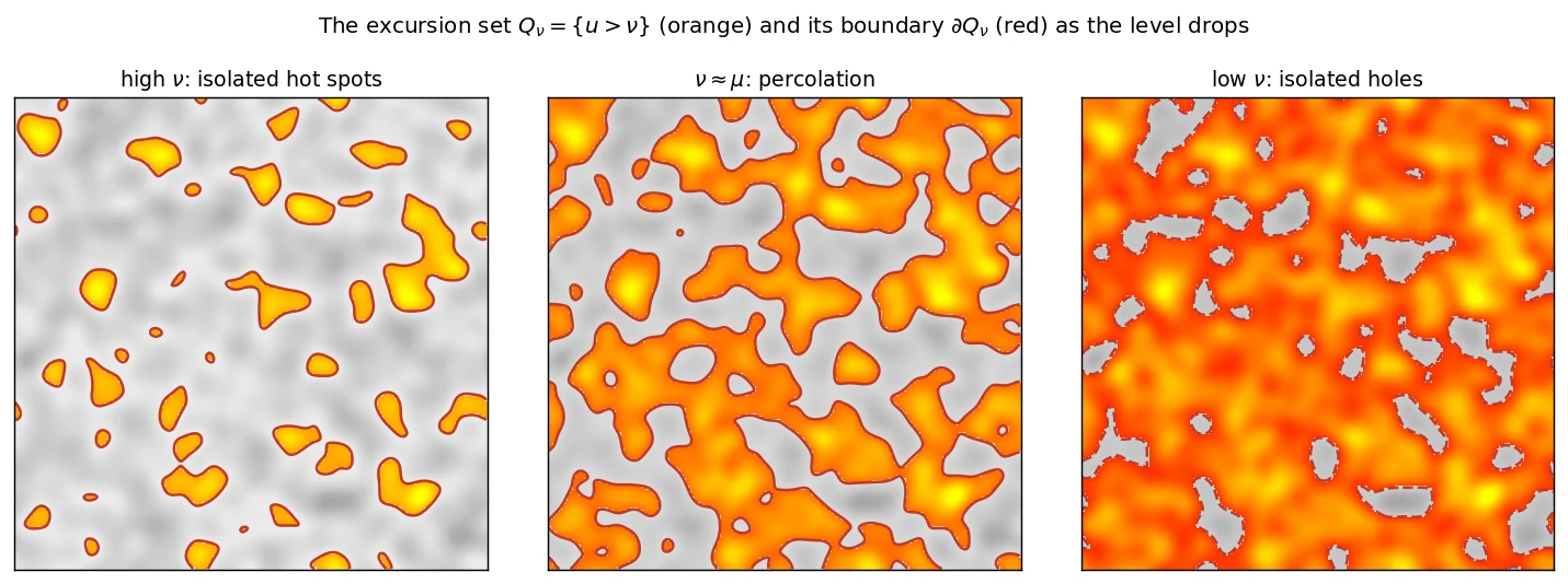
The same field flooded to three levels. Orange = land (Qν), red = coastline. Left: high water, isolated islands (χ>0, short coastline). Middle: percolation, one lacy continent (longest coastline, χ≈0). Right: low water, isolated lakes (χ<0).
Here is the structural point we'll exploit relentlessly. \(V_0\) depends only on the field's values (its one-point distribution), while \(V_1, V_2,\dots\) involve gradients and curvatures. The higher functionals probe how neighbouring points are correlated, which is genuine spatial structure invisible to the one-point histogram alone.
The Gaussian baseline and its Hermite structure
This is the section that turns Minkowski functionals into a measurement. A random field \(u(\mathbf x)\) attaches a random number to every point; it is Gaussian if every finite collection of values is jointly normal. The crucial consequence:
A Gaussian field is completely determined by its mean and its two-point correlation \(\xi(\mathbf x,\mathbf x')=\left\langle u(\mathbf x)u(\mathbf x') \right\rangle\), equivalently by its power spectrum \(P(k)\). Everything else is forced. In particular its Fourier phases are independent and random: no preferred patterns, no filaments, no clustering beyond what random phase-mixing produces. Correlated phases are exactly what "non-Gaussianity" means, and exactly what the power spectrum cannot see but Minkowski functionals can.
Spectral moments: the only two numbers that can appear
Because a Gaussian field is fixed by \(P(k)\), every ensemble-averaged MF must be an integral of \(P(k)\). The relevant integrals are the spectral moments \(\sigma_n^2=\int \frac{d^dk}{(2\pi)^d}\,k^{2n}P(k)\), and only the first two ever appear:
\[ \sigma_0^2=\left\langle u^2 \right\rangle\ \ (\text{field variance}),\qquad \sigma_1^2=\left\langle |\nabla u|^2 \right\rangle\ \ (\text{gradient variance}). \]
A gradient brings down one power of k (∂ → ik in Fourier space), so σ₁² carries a k² weight and σ₀² none. The ratio σ₁/σ₀ is an inverse coherence length: large for a wiggly small-scale field, small for a smooth one.
On the sphere (for the CMB), the same two numbers come from the angular power spectrum \(C_\ell\) and beam window \(b_\ell\): \(\sigma_0^2=\sum_\ell\frac{2\ell+1}{4\pi}b_\ell^2 C_\ell\) and \(\sigma_1^2=\sum_\ell\frac{2\ell+1}{4\pi}\ell(\ell+1)b_\ell^2 C_\ell\), where the spherical Laplacian eigenvalue \(\ell(\ell+1)\) plays the role of \(k^2\). As a feel for the ratio: a map dominated by power near \(\ell\approx150\) has \(\sigma_1/\sigma_0\approx\sqrt{150\cdot151}\approx150\) per radian, a coherence length of about \(1/150\) rad, or roughly \(0.4^\circ\).
We will write the threshold in rms units, \(\nu\to\nu/\sigma_0\), throughout.
\(V_0\) from first principles
\(V_0(\nu)\) is the fraction of space above threshold, i.e. the probability that a single Gaussian value exceeds \(\nu\):
\[ V_0(\nu)=\Pr[u\ge\nu]=\int_\nu^\infty\frac{e^{-u^2/2\sigma_0^2}}{\sqrt{2\pi}\,\sigma_0}\,du=\tfrac12\,\mathrm{erfc}\!\left(\frac{\nu}{\sqrt2\,\sigma_0}\right). \]This is the most familiar curve in the set: the Gaussian tail. Reading off a few thresholds makes it concrete.
| Threshold \(\nu/\sigma_0\) | \(V_0\) (fraction above) |
|---|---|
| \(0\) | \(0.500\) (half the map) |
| \(1\) | \(0.159\) |
| \(2\) | \(0.023\) (about 2.3%) |
| \(3\) | \(0.0013\) |
So at the \(2\sigma\) level only about one part in forty of the sky sits in hot spots, and by \(3\sigma\) it is barely one in a thousand. That steep tail is why the high-threshold MF curves are so noisy: there is hardly any land left to measure.
\(V_1\): the co-area trick, derived in full
Measuring the length of a wiggly coastline on a pixel grid sounds awful: the contour weaves between pixels and you never know exactly where it goes. The escape is the co-area formula, which converts a length integral that "lives on a 1D curve" into an area integral that "lives on the whole 2D map":
\[ \boxed{\;\underbrace{\int_{\partial Q_\nu}\!d\ell}_{\text{contour length}}=\underbrace{\int \delta\big(u(\mathbf x)-\nu\big)\,|\nabla u|\,d^2x}_{\text{area integral with a }\delta\text{ that picks the contour}}\;} \]It is worth deriving honestly, because the same machinery returns for \(V_2\). Picture the map as a topographic chart: \(u(\mathbf x)\) is altitude, the threshold \(\nu\) is a fixed contour line (say 1000 m), and the gradient \(\nabla u\) points up the steepest slope, perpendicular to the contour. Where the terrain is steep the contours bunch; where it is gentle they spread.

Concentric contours {u=ν}, {u=ν+Δν}, … The gradient ∇u points perpendicular to each contour. Steep terrain means contours close together; gentle terrain means contours spread apart.
Step 1: zoom until the contour looks straight. Pick a point \(P\) on the contour (\(u(P)=\nu\)) and zoom in below the contour's radius of curvature. Locally the contour is a straight line, the sphere is a flat plane, and \(\nabla u\) is a constant vector across it. Set up \(\xi\)along the contour and \(\eta\)across it (uphill, along \(\nabla u\)). Formally this is the implicit function theorem (\(\nabla u(P)\neq0\) implies smooth level sets), and locally the metric is Euclidean so \(dA=d\xi\,d\eta\).
Step 2: walking uphill, how fast does altitude rise? By definition \(|\nabla u|\) is the rate \(u\) climbs per unit distance along \(\eta\), so near \(P\), \(\,u(\xi,\eta)\approx \nu+|\nabla u|\,\eta\). Turning it around, to gain \(\Delta\nu\) in altitude you must walk
\[ \Delta\eta=\frac{\Delta\nu}{|\nabla u|} \]across the contour. That is the local thickness of the strip between the \(\nu\) and \(\nu+\Delta\nu\) contours: thin where steep, wide where gentle.


Left: the two contours are locally parallel, separated by Δν/|∇u| in the η direction. Right: the 1D ramp has slope |∇u|, so a rise Δν needs a step Δη = Δν/|∇u|.
Step 3: the strip is a ribbon, and its area is length times width. Zoom back out. The slab \(S_{\Delta\nu}=\{\mathbf x:\nu\le u\le\nu+\Delta\nu\}\) is a thin ribbon hugging the contour, of varying width \(\Delta\nu/|\nabla u|\). Summing length times width over the contour,
\[ \mathrm{Area}(S_{\Delta\nu})=\int_{\partial Q_\nu}\frac{\Delta\nu}{|\nabla u|}\,d\ell+O(\Delta\nu^2). \]
The slab SΔν is a ribbon hugging ∂Qν, of local width Δν/|∇u|: thin where steep, wider where gentle. Its area is ∫(Δν/|∇u|) dℓ along the contour.
Step 4: the same area, counted differently. The ribbon is also just "all points whose \(u\) falls in \([\nu,\nu+\Delta\nu]\)":
\[ \mathrm{Area}(S_{\Delta\nu})=\int \mathbf 1_{[\nu,\,\nu+\Delta\nu]}\big(u(\mathbf x)\big)\,d^2x. \]Step 5: shrink the ribbon to zero width. Equate the two expressions and divide by \(\Delta\nu\). The right side becomes \(1/\Delta\nu\) inside a window whose area stays \(1\), which is the defining bump-function construction of the Dirac delta, \(\lim_{\Delta\nu\to0}\mathbf 1_{[\nu,\nu+\Delta\nu]}(u)/\Delta\nu=\delta(u-\nu)\). So
\[ \int_{\partial Q_\nu}\frac{d\ell}{|\nabla u|}=\int \delta\big(u-\nu\big)\,d^2x. \]Step 6: clear the stray \(1/|\nabla u|\). Multiply the left integrand by \(|\nabla u|/|\nabla u|=1\) to move one factor across, and you land on the boxed co-area formula. The \(|\nabla u|\) is no fudge: it is the Jacobian of the change of variable \(u\leftrightarrow\eta\), the exchange rate that converts "length per unit altitude" into "length per unit distance." Drop it and you would be measuring the contour in the wrong units.
Now the expectation is easy. Under a Gaussian field \(u\) is independent of its gradient, so the average factorises into a one-point density and a mean gradient,
\[ \bar V_1(\nu)=\tfrac14\left\langle \delta(u-\nu) \right\rangle\,\left\langle |\nabla u| \right\rangle=\tfrac14\,p(\nu)\cdot\sqrt{\tfrac{\pi}{2}}\,\sigma_1 , \]where \(\left\langle |\nabla u| \right\rangle=\sqrt{\pi\tau/2}\) is the mean of a Rayleigh distribution (the modulus of a 2D Gaussian gradient, \(p_{|\nabla u|}(g)=\tfrac g\tau e^{-g^2/2\tau}\)). The same \(\nu\)-dependence drops out of Rice's formula for the level-crossing rate of a 1D Gaussian process, \(N^+(\nu)=\frac1{2\pi}\frac{\sigma_1}{\sigma_0}e^{-\nu^2/2\sigma_0^2}\), lifted to 2D contour length by Crofton's formula. Two roads to the same Gaussian bump.
\(V_2\): from geodesic curvature to a local invariant
The topological functional is the subtle one, and it repays a careful derivation. \(V_2\) integrates the geodesic curvature \(\kappa\) of the coastline,
\[ V_2(\nu)=\frac{1}{2\pi}\int_{\partial Q_\nu}\kappa\,d\ell, \]and by Gauss-Bonnet that integral is locked to the Euler characteristic. To take its Gaussian average we first need \(\kappa\) written as a local function of the field, with no explicit contour anywhere.
Walk along the coastline. The unit normal pointing uphill is \(\mathbf N=\nabla u/|\nabla u|\), and the geodesic curvature is the rate that normal turns, \(\kappa=-\nabla\!\cdot\!\mathbf N\). Carrying out that divergence and clearing the stray \(1/|\nabla u|\) with the same co-area trick that tamed \(V_1\), the boundary integrand becomes a pure ratio of derivatives:
\[ \kappa\,|\nabla u| \;=\; \frac{2\,u_x u_y\,u_{xy}-u_x^2\,u_{yy}-u_y^2\,u_{xx}}{u_x^2+u_y^2}. \]
Geodesic curvature κ is the turning rate of the tangent, the inverse radius of the osculating circle. It is positive when the contour curves away from ∇u (a convex hot spot, V₂>0) and negative when it curves toward ∇u (a concave hole, V₂<0).
Read the numerator out loud: it is the Hessian of \(u\) evaluated along the contour, in the one direction (perpendicular to \(\nabla u\)) that the level set is free to wiggle. It asks how the landscape bends in exactly the direction the coastline runs. So the expectation is again a single local average,
\[ \bar V_2(\nu)=\frac{1}{2\pi}\Big\langle\,\delta(u-\nu)\;\frac{2\,u_x u_y u_{xy}-u_x^2 u_{yy}-u_y^2 u_{xx}}{u_x^2+u_y^2}\,\Big\rangle, \]now a function of \(u\) and its first two derivatives, exactly the form a computer can accumulate pixel by pixel (we do precisely this when we build the estimator). The Gaussian average factorises one more time: \(u\) is independent of its derivatives, and in the frame where \(\nabla u\) lies along one axis the cross-terms vanish on average, collapsing the curvature integral to the classic Tomita result, an antisymmetric curve,
\[ \boxed{\; \bar V_2(\nu)=\frac{1}{(2\pi)^{3/2}}\,\frac{\tau}{\sigma}\,\frac{\nu-\mu}{\sqrt{\sigma}}\;e^{-(\nu-\mu)^2/2\sigma}. \;} \]This is the clean Hermite rung \(H_1\) (no spurious \(\sqrt2\)): positive above the mean (the excursion set is convex hot spots, the contour curves one way), negative below it (the excursion set is the sea around concave holes, the contour curves the other way), crossing zero exactly at percolation \(\nu=\mu\). That sign flip is the Euler characteristic changing sign, the hot-spot to cold-hole duality.

Why V₂ is antisymmetric. At high ν the excursion set is convex hot spots: walking the boundary with land on the left, the tangent turns through +2π, so ∮κ dℓ > 0 and V₂ > 0. At low ν it is the sea around cold holes: the tangent turns through −2π, so V₂ < 0. The crossover is percolation at ν = μ.
On the curved sphere the \(u_x,u_{xy},\dots\) become covariant derivatives, with the metric factors spelled out when we build the estimator, but the structure is identical. Morse theory gives the same antisymmetry from the other side: \(\chi(Q_\nu)=\#(\text{maxima})-\#(\text{saddles})+\#(\text{minima})\) above \(\nu\). Sweeping \(\nu\) down, isolated peaks appear first (\(+1\) each), then saddles bridge them (\(-1\)), then the deepest minima fill in. That competition draws the antisymmetric (2D) and W-shaped (3D) genus curves.
The unifying identity: a ladder of derivatives
Here is the punchline. The Hermite polynomials are generated by differentiating the Gaussian (Rodrigues' formula), \(H_n(\nu)\,e^{-\nu^2/2}=(-1)^n\frac{d^n}{d\nu^n}e^{-\nu^2/2}\), and the Minkowski functionals are exactly that ladder:
\[ \begin{aligned} V_0 &\propto \textstyle\int_\nu^\infty e^{-t^2/2}dt = \mathrm{erfc} &&(\text{antiderivative})\\ V_1 &\propto H_0\,e^{-\nu^2/2}=e^{-\nu^2/2} &&(H_0=1)\\ V_2 &\propto H_1\,e^{-\nu^2/2}=\nu\,e^{-\nu^2/2} &&(\text{2D Euler})\\ V_3 &\propto H_2\,e^{-\nu^2/2}=(\nu^2-1)\,e^{-\nu^2/2} &&(\text{3D genus}) \end{aligned} \qquad V_{k}\propto\Big(\tfrac{\sigma_1}{\sigma_0}\Big)^{k}H_{k-1}(\nu)\,e^{-\nu^2/2}. \]In one sentence: each higher Minkowski functional differentiates the Gaussian weight one more time, climbing the Hermite ladder and gaining one factor of \(\sigma_1/\sigma_0\) per rung. This is no accident of low dimension. It is the content of the Gaussian Kinematic Formula (Adler & Taylor): the expected MFs factor into [pure geometry of the survey region] times [universal Hermite times Gaussian threshold functions]. SymPy confirms the ladder:
import sympy as sp
nu = sp.symbols('nu', real=True); G = sp.exp(-nu**2/2)
for n in range(4):                              # Rodrigues' formula
    Hn = sp.expand(sp.simplify(sp.diff(G, nu, n)/G*(-1)**n))
    print(f"H_{n}(nu) =", Hn)
print("V1 ∝ H0 =", sp.expand(sp.simplify( sp.diff(G,nu,0)/G)))
print("V2 ∝ H1 =", sp.expand(sp.simplify(-sp.diff(G,nu,1)/G)))
print("V3 ∝ H2 =", sp.expand(sp.simplify( sp.diff(G,nu,2)/G)))
print("zeros of the 3D genus (H2=0):", sp.solve(nu**2-1, nu))
H_0(nu) = 1
H_1(nu) = nu
H_2(nu) = nu**2 - 1
H_3(nu) = nu**3 - 3*nu
V1 ∝ H0 = 1
V2 ∝ H1 = nu
V3 ∝ H2 = nu**2 - 1
zeros of the 3D genus (H2=0): [-1, 1]So the 2D Euler curve crosses zero at the mean, and the 3D genus crosses at \(\nu=\pm1\sigma\). These are universal predictions for any Gaussian field. Here are the shapes on one axis:

The Hermite ladder. V₁ (contour length) is a centred bump; V₂ (2D Euler) is odd, zero at ν=0; V₃ (3D genus) is even, dipping to −1 in the "sponge" regime and recovering in both tails, with zeros at ν=±1σ.
Exact formulas collected
The 2D Gaussian predictions (think of a CMB map), in the variance convention I verify below (\(\sigma=\sigma_0^2\), \(\tau=\tfrac12\sigma_1^2\), threshold \(\nu\) about the mean \(\mu\)):
\[ \boxed{\; \bar V_0=\tfrac12\Big[1-\mathrm{erf}\tfrac{\nu-\mu}{\sqrt{2\sigma}}\Big],\quad \bar V_1=\tfrac18\sqrt{\tfrac{\tau}{\sigma}}\,e^{-\frac{(\nu-\mu)^2}{2\sigma}},\quad \bar V_2=\tfrac{1}{(2\pi)^{3/2}}\tfrac{\tau}{\sigma}\tfrac{\nu-\mu}{\sqrt{\sigma}}\,e^{-\frac{(\nu-\mu)^2}{2\sigma}}. \;} \]Let's prove the two nontrivial Gaussian integrals (the \(V_0\) error function and the \(V_1\) Rayleigh mean gradient) with SymPy:
import sympy as sp
u, nu, mu = sp.symbols('u nu mu', real=True)
sigma = sp.Symbol('sigma', positive=True)   # VARIANCE
tau   = sp.Symbol('tau',   positive=True)    # gradient variance
g     = sp.Symbol('g', real=True)

p_u = 1/sp.sqrt(2*sp.pi*sigma)*sp.exp(-(u-mu)**2/(2*sigma))
print("normalisation:", sp.integrate(p_u, (u, -sp.oo, sp.oo)))
v0 = sp.simplify(sp.integrate(p_u, (u, nu, sp.oo)))
print("v0(nu) =", v0, " ; v0(mu) =", sp.simplify(v0.subs(nu, mu)))
p_ray = g/tau*sp.exp(-g**2/(2*tau))                    # Rayleigh pdf of |grad u|
mean_grad = sp.simplify(sp.integrate(g*p_ray, (g, 0, sp.oo)))
print("<|grad u|> =", mean_grad)
v1 = sp.simplify(sp.Rational(1,4)*p_u.subs(u, nu)*mean_grad)
target = sp.Rational(1,8)*sp.sqrt(tau/sigma)*sp.exp(-(nu-mu)**2/(2*sigma))
print("v1 matches boxed form?", sp.simplify(v1 - target) == 0)
print("dv0/dnu =", sp.simplify(sp.diff(v0, nu)))          # should be -p(nu)
normalisation: 1
v0(nu) = erf(sqrt(2)*(mu - nu)/(2*sqrt(sigma)))/2 + 1/2
v0(mu) = 1/2
<|grad u|> = sqrt(2)*sqrt(pi)*sqrt(tau)/2
v1 matches boxed form? True
dv0/dnu = -sqrt(2)*exp(-(mu - nu)**2/(2*sigma))/(2*sqrt(pi)*sqrt(sigma))v0 comes out as \(\tfrac12+\tfrac12\mathrm{erf}(\tfrac{\mu-\nu}{\sqrt{2\sigma}})\), which is the boxed form (erf is odd); the Rayleigh mean is \(\sqrt{\pi\tau/2}\); the boxed \(V_1\) checks out (v1 matches boxed form? True); and \(dV_0/d\nu=-p(\nu)\), so the area's slope is the boundary density. A second engine, WolframScript, agrees:
v0 = Integrate[Exp[-(u-m)^2/(2 s)]/Sqrt[2 Pi s], {u, nu, Infinity}, Assumptions -> s>0];
Print["v0 = ", Simplify[v0], " ; v0(m) = ", Simplify[v0 /. nu->m]];
meanGrad = Integrate[g (g/t) Exp[-g^2/(2 t)], {g, 0, Infinity}, Assumptions -> t>0];
v1 = (1/4)(Exp[-(nu-m)^2/(2 s)]/Sqrt[2 Pi s]) meanGrad;
Print["match v1? = ", Simplify[v1 - (1/8) Sqrt[t/s] Exp[-(nu-m)^2/(2 s)] == 0, Assumptions->{s>0,t>0}]];
v0 = (1 + Erf[(m - nu)/(Sqrt[2] Sqrt[s])])/2 ; v0(m) = 1/2
<|grad u|> = Sqrt[Pi/2] Sqrt[t]
match v1? = TrueIn 3D the ladder adds the genus \(\;\bar V_3\propto(\sigma_1/\sigma_0)^3(\nu^2-1)\,e^{-\nu^2/2}\), the famous \((\nu^2-1)\) shape Gott, Melott & Dickinson used for galaxy surveys.
Measuring the functionals on a pixel grid
We have the closed-form curves. Before we can compare anything to them, we need to estimate the same curves from a finite, masked map of pixel values. The trick (Schmalzing & Górski 1998) is to never trace a contour at all. Write each functional as a volume integral of a local invariant of the field and its derivatives, then sum it pixel by pixel. With \(G=|\nabla u|\) and the curvature combination \(H\) from the \(V_2\) derivation,
\[ v_0(\nu)=\big\langle\Theta(u-\nu)\big\rangle,\quad v_1(\nu)=\tfrac14\big\langle\delta(u-\nu)\,G\big\rangle,\quad v_2(\nu)=\tfrac1{2\pi}\big\langle\delta(u-\nu)\,H\big\rangle, \]and the Euler characteristic is assembled from the two via Gauss-Bonnet, \(\chi(\nu)=4\pi\,v_2(\nu)+2\,v_0(\nu)\) on the unit sphere. Each of those three lines hides a small story, because this is where the clean continuum formulas meet a finite grid.
\(v_0\) exactly: a sorted-array trick
\(v_0(\nu)\) is just "what fraction of unmasked pixels exceed \(\nu\)." Counting that for all \(31\) thresholds with a naive double loop is \(O(N\,N_\nu)\sim3\times10^7\) comparisons. Instead you sort the pixels once and binary-search each threshold:
u_sorted = np.sort(u_masked)                     # O(N log N), done once
idx      = np.searchsorted(u_sorted, nu_grid, side='left')
v0       = (N - idx) / N                          # fraction above each threshold
Worked example: six pixels \((0.5,0.1,0.7,0.3,0.9,0.2)\) at \(\nu=0.4\). Sorting gives \((0.1,0.2,0.3,0.5,0.7,0.9)\); searchsorted finds \(\nu=0.4\) slots in at index \(3\) (three values below it), so \(v_0=(6-3)/6=0.5\).

searchsorted on the sorted array: ν=0.4 splits 3 values below from 3 above, so v₀=3/6. Because a pixel is strictly above or below, with no "partial credit", v₀ has no bin-width bias; it is the exact empirical complementary CDF.
\(v_1\) and \(v_2\): a binned delta and a Goldilocks bin width
For \(v_1,v_2\) the integrand carries a \(\delta(u-\nu)\), which a finite grid cannot represent. Replace it by a top-hat of width \(\Delta\nu\) and height \(1/\Delta\nu\) (unit area preserved): every pixel whose value lands in bin \(k\) contributes its local invariant with weight \(1/\Delta\nu\). The discrete estimators are then \(v_1(\nu_k)=\tfrac1{4N\Delta\nu}\sum_{i\in k}G_i\) and \(v_2(\nu_k)=\tfrac1{2\pi N\Delta\nu}\sum_{i\in k}H_i\).


Left: the Dirac δ becomes a finite top-hat of width Δν, height 1/Δν. Right: 31 sample thresholds over μ ± 3.5√σ; each pixel value drops into one bin and adds its gradient (for v₁) or curvature invariant (for v₂).
Choosing \(\Delta\nu\) is the histogram-bin dilemma. Make the bins too narrow and each catches too few pixels: the expected count is \(n_{\rm bin}=N\,p(\nu_k)\,\Delta\nu\), so the shot noise is \(\sim1/\sqrt{n_{\rm bin}}\), worst in the tails where \(p(\nu_k)\) is tiny. Make them too wide and the top-hat averages the curve over a window broader than its own features, a binning bias \(\sim\Delta\nu/\sqrt\tau\).


Left: near the mean a bin holds many pixels (low shot noise); in the tail it holds few. Right: too few bins miss the peak (bias), too many bounce around it (shot noise); 31 bins (≈0.23√σ) keep both sub-percent.
With \(\sim\!10^6\) masked pixels and \(\tau\gtrsim10^4\sigma\), the choice \(\Delta\nu\approx0.23\sqrt\sigma\) from \(N_\nu=31\) lands in the Goldilocks zone: shot noise \(\sim1.5\%\) at the very tails, binning bias \(\sim2\times10^{-3}\), both well below a percent everywhere it matters.
The derivatives are covariant, and healpy already has them
One subtlety hides in \(G_i=|\nabla u|\) and the curvature invariant \(H_i\): on the sphere these are covariant derivatives, not naive finite differences. In the orthonormal frame of the metric \(ds^2=d\vartheta^2+\sin^2\!\vartheta\,d\varphi^2\) the first derivatives are
\[ u_{;\vartheta}=\partial_\vartheta u,\qquad u_{;\varphi}=\frac1{\sin\vartheta}\,\partial_\varphi u, \]and the second derivatives pick up Christoffel corrections,
\[ u_{;\vartheta\vartheta}=\partial_\vartheta^2u,\quad u_{;\vartheta\varphi}=\tfrac1{\sin\vartheta}\partial_\vartheta\partial_\varphi u-\cot\vartheta\,u_{;\varphi},\quad u_{;\varphi\varphi}=\tfrac1{\sin^2\vartheta}\partial_\varphi^2u+\cot\vartheta\,u_{;\vartheta}. \]The lovely part: healpy.alm2map_der1 returns \(\partial_\vartheta u\) and \(\tfrac1{\sin\vartheta}\partial_\varphi u\), which are exactly the covariant first derivatives. Feed those two maps back through alm2map_der1 a second time and you get every second derivative. The \(u_{;\vartheta\varphi}\) correction cancels automatically (the \(1/\sin\vartheta\) is already baked into d_phi), and only \(u_{;\varphi\varphi}\) needs a single \(+\cot\vartheta\,u_{;\vartheta}\) term. That is the covariant_derivatives function we run next.
The fit: measure all four functionals and overlay the theory
Symbolic checks confirm the algebra; now confirm the measurement, with the real estimator cosmologists run on the sky rather than a toy. We wire the pieces from the last section together, simulate a Gaussian field on the sphere with a known spectrum, measure \((\sigma,\tau)\) from its pixels, and overlay the closed forms with nothing else fitted:
import numpy as np, healpy as hp
from scipy.special import erf

NSIDE, LMAX = 256, 512
ell = np.arange(LMAX+1)
Cl = np.exp(-(ell/45.0)**2); Cl[0]=Cl[1]=0          # smooth, band-limited spectrum

def covariant_derivatives(u):                        # SG convention, via two der1 passes
    alm = hp.map2alm(u, lmax=LMAX, iter=3)
    _, u_t, u_p = hp.alm2map_der1(alm, NSIDE, lmax=LMAX)        # u_;θ , u_;φ
    theta, _ = hp.pix2ang(NSIDE, np.arange(hp.nside2npix(NSIDE)))
    cot = np.cos(theta)/np.maximum(np.sin(theta), 1e-9)
    _, u_tt, _      = hp.alm2map_der1(hp.map2alm(u_t, lmax=LMAX, iter=3), NSIDE, lmax=LMAX)
    _, u_tp, u_ppr  = hp.alm2map_der1(hp.map2alm(u_p, lmax=LMAX, iter=3), NSIDE, lmax=LMAX)
    return u_t, u_p, u_tt, u_tp, u_ppr + cot*u_t     # the one connection correction

nu_x = np.linspace(-3.5, 3.5, 31)                    # thresholds in units of sqrt(sigma)
acc = {k: np.zeros(31) for k in ("v0","v1","v2")}; Sg = Tau = 0.0
for _ in range(6):                                   # average a few realisations
    m = hp.synfast(Cl, NSIDE, lmax=LMAX, new=True); m -= m.mean()
    u_t, u_p, u_tt, u_tp, u_pp = covariant_derivatives(m)
    sigma, tau = m.var(), 0.5*np.mean(u_t**2 + u_p**2)          # the only two numbers
    Sg += sigma; Tau += tau
    nu = nu_x*np.sqrt(sigma); dnu = nu[1]-nu[0]; N = m.size
    G = np.sqrt(u_t**2 + u_p**2)                                # |grad u|
    H = (2*u_t*u_p*u_tp - u_t**2*u_pp - u_p**2*u_tt)/(G**2)     # curvature invariant
    acc["v0"] += [np.mean(m > t) for t in nu]                  # exact complementary CDF
    k = np.floor((m - (nu[0]-dnu/2))/dnu).astype(int); ok = (k>=0)&(k<31)
    b = np.zeros(31); np.add.at(b, k[ok], G[ok]); acc["v1"] += b/(4*N*dnu)
    b = np.zeros(31); np.add.at(b, k[ok], H[ok]); acc["v2"] += b/(2*np.pi*N*dnu)

v0,v1,v2 = (acc[k]/6 for k in ("v0","v1","v2")); sigma,tau = Sg/6, Tau/6
chi = 4*np.pi*v2 + 2*v0

nu = nu_x*np.sqrt(sigma); g = np.exp(-nu**2/(2*sigma))         # Tomita closed forms
v0_G = 0.5*(1 - erf(nu/np.sqrt(2*sigma)))
v1_G = (1/8)*np.sqrt(tau/sigma)*g
v2_G = (1/(2*np.pi)**1.5)*(tau/sigma)*(nu/np.sqrt(sigma))*g
chiG = 4*np.pi*v2_G + 2*v0_G

# one peak-normalised number per curve: the non-Gaussianity score
for nm,a,t in [("v0",v0,v0_G),("v1",v1,v1_G),("v2",v2,v2_G),("chi",chi,chiG)]:
    print(f"chi2_{nm} = {np.mean(((a-t)/np.max(np.abs(t)))**2):.1e}")
measured sigma = 163.3 tau = 1.68e5 sqrt(tau/sigma) = 32.1
chi2_v0 = 3.8e-07
chi2_v1 = 5.8e-06
chi2_v2 = 5.6e-05
chi2_chi = 5.6e-05Two numbers, \(\sigma\) and \(\tau\), measured straight from the pixels, and all four closed-form curves drop on top of the data with nothing else fitted:

The fit, functional by functional. Top: measured (orange) on the Tomita Gaussian expectation (blue) for the four curves; bottom: the fractional residual, with the grey band at ±5%. Built from the gold-standard Schmalzing-Górski estimator on the sphere, the same code that runs on Planck maps.
Now read the panels, because each one teaches a different lesson. This is the intuition the curves were built to give:
\(v_0\), the area function, is exact. It only ever asks "is this pixel above \(\nu\)?", so it is the empirical complementary CDF of the one-point histogram with no bin-width approximation, and it tracks \(\tfrac12\,\mathrm{erfc}\) to \(\sim\!10^{-7}\). It depends on the field's values alone and is blind to spatial structure.
\(v_1\), the coastline, is the first-derivative test. Its Gaussian peak sits exactly at \(\nu=\mu\) and its height is \(\tfrac18\sqrt{\tau/\sigma}\), the only place the gradient scale \(\sqrt{\tau/\sigma}\) enters. The fit is good to \(\sim\!10^{-6}\) because a smooth field's mean gradient is a stable, well-sampled quantity.
\(v_2\) and \(\chi\), the curvature and topology curves, are the delicate ones. They ride on second derivatives, which weight the small scales hardest, so they are the noisiest and most demanding to get right (here \(\sim\!10^{-5}\), on real masked data \(\sim\!10^{-3}\)). They are antisymmetric about the mean, crossing zero at percolation. That is exactly why cosmologists prize them: the most fragile curve carries the richest morphology.
The amplitude that matters is \(\sqrt{\tau/\sigma}\). Everything else in the four shapes is universal, a parameter-free prediction of Gaussianity. A small but real subtlety lives here: the curvature panel matches the clean Hermite rung \(H_1\propto(\nu-\mu)/\sqrt\sigma\), not the \(\sqrt2\)-shifted form that sometimes appears in notes, and the estimator settles the convention to \(10^{-5}\).
The takeaway: feed in a Gaussian field, and four independent estimators (counting, gradients, curvature, topology) all snap onto closed-form Hermite times Gaussian curves with two measured numbers. Any field that fails to do this is announcing non-Gaussianity. The rest of the post is about reading that failure.
Why this matters: what the power spectrum cannot see
Minkowski functionals earn their place in cosmology for four reasons.
They give an exact, almost parameter-free null test. The Gaussian curves above are predicted exactly, with only the amplitude \(\sigma_1/\sigma_0\) fitted. Any departure of the measured \(V_k(\nu)\) from the Hermite times Gaussian shapes is a model-independent flag of non-Gaussianity.
They carry information the power spectrum is blind to. \(C_\ell\) captures only the two-point function, which is identical for a true Gaussian field and for any field with the same spectrum but scrambled phases. MFs are built from the geometry of iso-contours, so they are sensitive to phase correlations, the whole hierarchy of higher-order connected correlations.
They make a sharp foreground diagnostic. A clean CMB map should obey the Gaussian predictions, while Galactic dust and other foregrounds are markedly non-Gaussian and distort the curves in characteristic ways. That is a direct test of component-separation pipelines.
They are cheap and robust. Additivity (M2) means MFs compute by simple local algorithms on a HEALPix map, accumulating cell by cell, and they hold up against noise better than high-order \(n\)-point estimators.
The second point deserves a concrete thought experiment. Construct two CMB-like maps. Map A is a genuine Gaussian realisation of the Planck best-fit \(C_\ell\), with independent random harmonic phases. Map B is a non-Gaussian map (say a lognormal model or an \(f_{\rm NL}=50\) simulation); measure its \(|a_{\ell m}|\) but replace the phases with Map A's. By construction Maps A and B have identical \(C_\ell\), since \(C_\ell\propto\langle|a_{\ell m}|^2\rangle\). A power-spectrum measurement cannot tell them apart. The MFs instantly do: Map B has excess clustering of hot spots, its genus curve departs from the template, and its zero-crossings shift. MFs and power spectra are complementary, not competing. The spectrum fully describes a Gaussian field, and for a non-Gaussian one the MFs read the extra information stored in phases, compressed into three scalar curves.
Non-Gaussianity: how the curves shift
The local-model primordial potential gets a quadratic correction \(\Phi=\varphi_G+f_{\rm NL}\,[\varphi_G^2-\langle\varphi_G^2\rangle]\), so \(f_{\rm NL}\) controls the skewness of the one-point PDF. Its effect on the curves:
\(f_{\rm NL}>0\) gives a positive skew: rare high peaks are enhanced, the genus/Euler curve shifts to larger \(\nu\), and \(V_0\) departs from erfc in the tail.
\(f_{\rm NL}<0\) gives a negative skew: peaks are suppressed, troughs enhanced.
\(f_{\rm NL}=0\) is exact Gaussian: all functionals follow the Hermite times Gaussian templates.

Schematic non-Gaussian deviation of the 2D Euler curve. Because the Gaussian shape is predicted exactly, any systematic departure is an unambiguous morphological detection of non-Gaussianity, independent of the power spectrum.
Matsubara (2003, 2010) computed the leading correction perturbatively. Defining three skewness parameters \(S^{(0)}=\langle u^3\rangle/\sigma_0^4\), \(S^{(1)}=\langle u^2\nabla^2u\rangle/(\sigma_0^2\sigma_1^2)\), \(S^{(2)}=\langle(\nabla u)^2\nabla^2u\rangle/\sigma_1^4\), the corrected functionals read \(V_k=V_k^{\rm G}\,[1+\sigma_0(a_kS^{(0)}+b_kS^{(1)}+c_kS^{(2)})]+\mathcal O(\sigma_0^2)\) with known Hermite coefficients \(a_k,b_k,c_k\). For primordial non-Gaussianity \(S^{(0)}\propto f_{\rm NL}\), so fitting yields a direct constraint on \(f_{\rm NL}\).
These skewness parameters are weighted projections of the bispectrum \(B(k_1,k_2,k_3)\), the connected three-point function \(\langle\delta_{\mathbf k_1}\delta_{\mathbf k_2}\delta_{\mathbf k_3}\rangle_c\). Translational invariance forces \(\mathbf k_1+\mathbf k_2+\mathbf k_3=0\), so the three wavevectors form a closed triangle, and the shape of that triangle encodes the physics:
| Triangle | Configuration | Physical origin |
|---|---|---|
| Squeezed (\(k_1\ll k_2\approx k_3\)) | one long, two short | multi-field inflation; a superhorizon mode modulates small-scale power |
| Equilateral (\(k_1\approx k_2\approx k_3\)) | all equal | non-standard kinetic term; modes leave the horizon together |
| Folded (\(k_1+k_2\approx k_3\)) | two nearly collinear | non-Bunch-Davies initial state |
Because local, equilateral, and folded bispectra peak at different triangle shapes, the three skewness parameters (and their momentum-resolved cousins, the skew-spectra \(S^{(j)}(k)\) of Pratten & Munshi 2012) receive them in different ratios. Measuring all three MFs therefore constrains the shape of non-Gaussianity, not just its amplitude. One caution for large-scale structure: even with Gaussian initial conditions, nonlinear gravitational clustering generates its own bispectrum (the \(F_2\) mode-coupling kernel), about two orders of magnitude larger than a primordial \(f_{\rm NL}\sim20\) signal, and it must be subtracted before constraining \(f_{\rm NL}\).
A real application: is a dust-cleaned sky Gaussian?
Toy fields are reassuring, but a real analysis is the point. Here is one where these four curves do honest work. To see the cosmic microwave background or the cosmic infrared background, you must first scrub away the Galactic dust that glows in the same far-infrared bands. A standard way to do it is to fit each Planck map (\(217\), \(353\), \(545\,\)GHz) as a linear combination of neutral-hydrogen (\(\mathrm{HI}\)) templates, since dust traces gas, and subtract the fitted model. What is left is the residual
\[ r(\hat{\mathbf n})=d_\nu(\hat{\mathbf n})-\big[\bar O+\bar\varepsilon_{\rm LVC}(\hat{\mathbf n})\,T_{\rm LVC}(\hat{\mathbf n})+\bar\varepsilon_{\rm IVC}(\hat{\mathbf n})\,T_{\rm IVC}(\hat{\mathbf n})\big], \]where the offset \(\bar O\) and the per-region emissivities \(\bar\varepsilon\) come from a Bayesian (HMC) fit. If the fit worked, \(r\) should be nothing but CIB plus instrument noise, a Gaussian field. The usual check is the cross-power \(\rho_\ell^{r\times\mathrm{HI}}\), and indeed it comes out \(\lesssim0.1\). But a cross-correlation only tests linear coupling to the template at each scale. It can sit at zero while the residual still hides dust filaments, CO-bright clumps, or sharp phase edges, which are compact non-Gaussian features that integrate away in any two-point statistic. That is exactly the blind spot Minkowski functionals were built to cover.
The pipeline is the estimator we built above, applied to the masked residual. We measure \((\mu,\sigma,\tau)\) directly from the unmasked pixels, compute \(v_0\) from the sorted-array CDF, \(v_1\) and \(v_2\) from the binned local invariants, and assemble \(\chi=4\pi v_2+2v_0\). Then we condense each curve to a single non-Gaussianity score, its mean squared distance from the Gaussian expectation, normalised to the curve's own peak,
\[ \chi^2_j=\frac1{N_\nu}\sum_{k}\Big[\frac{v_j(\nu_k)-\bar v_j^{\,G}(\nu_k)}{\max_k|\bar v_j^{\,G}(\nu_k)|}\Big]^2. \]Two unrelated \(\chi\)'s collide here: the curve \(\chi(\nu)\) is the Euler characteristic, while the score \(\chi^2_j\) is one number per map per functional. A score of \(\chi^2_j=0.01\) would mean the curve typically misses Gaussian by \(\sqrt{0.01}=10\%\) of its height. Nine maps (three frequencies times three \(\mathrm{HI}\)-column masks) give nine times four such scores:

Every residual map is morphologically Gaussian. The four functionals climb a clean sensitivity ladder (χ²v₀ < χ²v₁ < χ²v₂≈χ²χ), and even the most sensitive curve sits 1.5 to 4 orders of magnitude below where an injected fNL∼100 non-Gaussianity would land.
Three patterns fall out, and each is a physical statement rather than a plotting artefact.
First, the residual is Gaussian to better than \(0.3\%\). All thirty-six scores lie between \(10^{-5}\) and \(3.3\times10^{-3}\). A hand-injected \(f_{\rm NL}\sim100\) would give \(\chi^2\sim0.1\), three orders of magnitude larger. So the morphology test independently confirms what the cross-power suggested: the dust fit really did leave behind only Gaussian CIB plus noise.
Second, there is a clear sensitivity hierarchy \(\chi^2_{v_0}<\chi^2_{v_1}<\chi^2_{v_2}\). The area function \(v_0\) (one-point values) matches to \(\sim\!10^{-5}\); \(v_1\) (first derivatives) deviates at \(\sim\!10^{-4}\); \(v_2\) and \(\chi\) (second derivatives) deviate at \(\sim\!10^{-3}\). The deeper into the field's derivative structure a functional reaches, the more of the multi-point hierarchy it can see, and the harder it is to fool. That is the whole reason to measure more than \(v_0\).
Third, \(217\) and \(353\,\)GHz improve as the mask tightens, but \(545\) does not. Clipping the brightest \(\mathrm{HI}\) regions drives \(\chi^2_{v_2}\) down monotonically at the two lower frequencies (\(3.1\to1.9\to1.7\times10^{-3}\) at \(217\)). At \(545\,\)GHz, where dust is about \(30\) times brighter, the trend stalls: a linear two-template model leaves small morphological residuals the mask cannot fully excise. The MFs are quietly pointing at the one band that wants a non-linear, spatially-varying-\(\beta_d\) dust model, a diagnosis the power spectrum simply cannot make.
Cross-power and Minkowski functionals are orthogonal tests, one for linear template correlation at fixed scale, the other for global Gaussianity at fixed threshold, and the residual passes both, at the \(\lesssim5\%\) and \(\lesssim0.3\%\) levels respectively, across all nine maps. Together they are a far stronger validation of the dust subtraction than either alone.
The CMB as a worked example
The CMB temperature map is the ideal testing ground: close to Gaussian, two-dimensional (the celestial sphere), and predicted by inflation with remarkable precision. Let \(u(\hat{\mathbf n})=\delta T/T\). After smoothing to a beam scale (Planck's \(5'\), say), one finds roughly \(\sigma_0\approx70\,\mu\)K and effective multipole \(\ell_{\rm eff}=\sigma_1/\sigma_0\approx100\) to \(200\). Each functional has a clean reading:
\(V_0\) is the area fraction of sky hotter than \(\nu\sigma_0\). At \(\nu=2\), \(V_0=\tfrac12\mathrm{erfc}(2/\sqrt2)\approx2.3\%\) of the sky sits in hot spots.
\(V_1\) is the total contour length of the \(\nu\sigma_0\) temperature contour, peaking at \(\nu=0\) along the longest hot-to-cold "cosmic equator." Any asymmetry between \(\nu>0\) and \(\nu<0\) flags non-Gaussianity or a systematic.
\(V_2\) is the genus, hot spots minus holes per unit area. As \(\nu\) drops you pass from isolated cold voids (\(\chi>0\)) to a multiply-connected sponge (\(\chi<0\)) to isolated hot spots (\(\chi>0\)). The zero-crossings at \(\nu=\pm\sigma_0\) are universal Gaussian predictions.

The genus journey, V₃ ∝ (ν²−1)e^(−ν²/2): isolated clusters at high ν (χ>0), a multiply-connected sponge for |ν|<1σ (χ<0), and isolated voids at low ν (χ>0). The zeros at ν=±1σ are predicted for any Gaussian field.
On a pixelised HEALPix map the standard Schmalzing-Górski estimators are exactly the local sums we used numerically, with the gradient and curvature built from covariant derivatives on the sphere. Two practical notes from the literature. A finite threshold bin introduces a systematic residual \(\propto(\Delta\nu)^2/\sigma_0\) in \(V_1,V_2\) (Lim & Simon 2012), which is a finite-difference effect rather than a pixelisation one, curable by integrating analytically over each bin. And for parameter inference one builds a Gaussian likelihood over the stacked MF vector with a simulation covariance and the Hartlap inverse-covariance debiasing \(C^{-1}\to\frac{N_{\rm sim}-p-2}{N_{\rm sim}-1}\hat C^{-1}\).
Representative MF-based constraints on primordial non-Gaussianity, all consistent with \(f_{\rm NL}=0\):
| Statistic / dataset | Constraint | Reference |
|---|---|---|
| Genus curve, WMAP 9-yr | \(\lvert f_{\rm NL}^{\rm local}\rvert\lesssim30\) | Hikage et al. 2008 |
| Combined \(V_0,V_1,V_2\), Planck 2018 | Gaussian at \(2\sigma\) | Planck Collab. 2020 |
| \(V_2\) + power spectrum, Planck 2018 | \(f_{\rm NL}^{\rm local}=-0.9\pm5.1\) | Planck Collab. 2020 |
| MFs, large-scale structure | \(\lvert f_{\rm NL}\rvert\lesssim50\) | Appleby et al. 2021 |
A modern refinement (Hamann & Kang 2023) beats the one-scale parameter degeneracy, where many spectra share the same \(\sigma_0,\sigma_1\), by needlet band-pass filtering the map and computing MFs scale by scale. Applied to the Planck lensing-convergence map, the MF-inferred \(\Omega_m h^2, A_s\) are fully consistent with the lensing power spectrum, an independent morphological cross-check that should tighten below the power spectrum once future surveys lower the noise.
The whole story in eight lines
Morphology is a coordinate-free description of size, shape, and connectivity.
Demand three things of a shape number: motion invariance, additivity, continuity.
Hadwiger (1957): in \(d\) dimensions exactly \(d+1\) such numbers exist, the Minkowski functionals, a complete basis.
Steiner picture: inflate the body by \(\varepsilon\); the volume is a polynomial in \(\varepsilon\) whose coefficients are the functionals.
Curvature picture: they are integrals of \(1\), surface element, mean curvature, Gaussian curvature, giving content, surface, bending, and topology (\(\chi\) via Gauss-Bonnet).
Excursion sets: threshold a random field at level \(\nu\) and measure the MFs of the dry land; sweep \(\nu\) to get curves \(V_k(\nu)\).
Gaussian baseline: \(V_k\propto(\sigma_1/\sigma_0)^k H_{k-1}(\nu)\,e^{-\nu^2/2}\), universal Hermite times Gaussian shapes, exact and parameter-free.
Payoff: deviations measure non-Gaussianity, the phase information the power spectrum cannot see, and diagnose foregrounds and systematics.
Guide to the literature
Hadwiger (1957) for the completeness theorem · Steiner (1840) for the parallel-body formula · Tomita (1986) for the Gaussian MF formulae · Gott, Melott & Dickinson (1986) for the genus statistic · Mecke et al. (1994) for MFs in cosmology · Schmalzing & Buchert (1997) and Schmalzing & Górski (1998) for practical estimators and the sphere · Adler & Taylor (2007), Random Fields and Geometry, for the Gaussian Kinematic Formula · Matsubara (2003, 2010) for perturbative non-Gaussian corrections and \(f_{\rm NL}\) · Lim & Simon (2012) for binning residuals · Pratten & Munshi (2012) for skew-spectra · Planck Collaboration (2020) for CMB MF measurements · Hamann & Kang (2023) for the needlet MF likelihood.
Flood responsibly. 🌊