
The Expanding Universe II — Kinematics
Part 2 of five. With the Robertson–Walker stage from Part 1 built, we now derive how light and free particles move on it — and find the two consequences of expansion: redshift and a surprisingly subtle notion of distance.
Everything we know about the universe arrives as light, so we need the equation of motion of photons and free particles in the expanding spacetime. That equation is the geodesic equation, and we derive it before applying it.
Geodesics — derived from a Lagrangian
A freely-falling particle extremises its proper time; equivalently, in a space with metric \(g_{ij}\) it extremises the action of the Lagrangian
\[ L = \tfrac12\,m\,g_{ij}(x)\,\dot x^i\dot x^j .\]Feed this to the Euler–Lagrange equation \(\frac{\mathrm d}{\mathrm d t}\big(\partial L/\partial\dot x^k\big)=\partial L/\partial x^k\). The right side is \(\tfrac12 m\,\partial_k g_{ij}\,\dot x^i\dot x^j\). The left side, using \(\frac{\mathrm d}{\mathrm d t}g_{ik}=\partial_j g_{ik}\,\dot x^j\), is
\[ \frac{\mathrm d}{\mathrm d t}\big(m\,g_{ik}\dot x^i\big) = m\,g_{ik}\ddot x^i + m\,\partial_j g_{ik}\,\dot x^i\dot x^j = m\,g_{ik}\ddot x^i + \tfrac12 m(\partial_j g_{ik}+\partial_i g_{jk})\dot x^i\dot x^j . \]Equating the two and multiplying by the inverse metric \(g^{lk}\) gives the geodesic equation
\[ \boxed{\;\frac{\mathrm d^2 x^l}{\mathrm d t^2} = -\,\Gamma^l_{ij}\,\dot x^i\dot x^j\;}, \qquad \Gamma^l_{ij} \equiv \tfrac12\,g^{lk}\big(\partial_i g_{jk} + \partial_j g_{ik} - \partial_k g_{ij}\big) .\]The Christoffel symbols \(\Gamma\) are the fictitious forces of curved coordinates — the same terms that make a straight line look bent in polar coordinates. Promoted to spacetime and written with the four-momentum \(P^\mu\), the geodesic equation is \(P^\alpha\nabla_\alpha P^\mu=0\), and it holds for massless particles too (the massive derivation via proper time simply carries over).
Applying it to FRW: energy redshifts as \(1/a\)
Take the RW metric \(\mathrm d s^2 = -c^2\mathrm d t^2 + a^2\gamma_{ij}\mathrm d x^i\mathrm d x^j\). We need its Christoffels. As an example, compute \(\Gamma^0_{\alpha\beta}=\tfrac12 g^{0\lambda}(\partial_\alpha g_{\beta\lambda}+\partial_\beta g_{\alpha\lambda}-\partial_\lambda g_{\alpha\beta})\). Only \(\lambda=0\) contributes (\(g^{00}=-1\)), and with \(g_{00}\) constant this reduces to \(\Gamma^0_{\alpha\beta}=\tfrac12\partial_0 g_{\alpha\beta}\). Non-zero only for spatial indices, where \(g_{ij}=a^2\gamma_{ij}\):
\[ \Gamma^0_{ij} = c^{-1}a\dot a\,\gamma_{ij} , \qquad \Gamma^i_{0j} = c^{-1}\frac{\dot a}{a}\,\delta^i_j .\]Now the geodesic equation for the energy. Homogeneity kills spatial gradients (\(\partial_i P^\mu=0\)), so \(P^0\,\mathrm d P^\mu/\mathrm d x^0 = -\Gamma^\mu_{\alpha\beta}P^\alpha P^\beta\). The \(\mu=0\) component, with \(P^0=E/c\) and \(\Gamma^0_{ij}\) from above, is
\[ \frac{E}{c^3}\frac{\mathrm d E}{\mathrm d t} = -\frac1c\,a\dot a\,\gamma_{ij}P^iP^j .\]For a massless particle the null constraint \(g_{\mu\nu}P^\mu P^\nu=0\) reads \(-c^{-2}E^2+a^2\gamma_{ij}P^iP^j=0\), so \(a^2\gamma_{ij}P^iP^j=E^2/c^2\). Substitute:
\[ \frac{E}{c^3}\frac{\mathrm d E}{\mathrm d t} = -\frac{\dot a}{a}\,\frac{E^2}{c^3} \;\Longrightarrow\; \boxed{\;\frac1E\frac{\mathrm d E}{\mathrm d t} = -\frac{\dot a}{a} \;\Longrightarrow\; E \propto a^{-1}.\;}\]A photon's energy decays as the universe expands. Repeating the exercise for a massive particle (constraint \(g_{\mu\nu}P^\mu P^\nu=-m^2c^2\)) gives the physical momentum \(p\propto a^{-1}\) as well — so free particles lose peculiar velocity and settle onto the Hubble flow. This one line is the engine of the hot Big Bang: everything cools as \(1/a\).
Redshift
Since \(E=hc/\lambda\) and \(E\propto a^{-1}\), wavelength stretches with the universe, \(\lambda\propto a\). Light emitted at \(t_1\) and observed at \(t_0\) therefore satisfies \(\lambda_0/\lambda_1=a(t_0)/a(t_1)\). Defining the redshift as the fractional stretch \(z\equiv(\lambda_0-\lambda_1)/\lambda_1\) and using \(a(t_0)\equiv1\),
\[ \boxed{\;1+z = \frac{1}{a(t_1)}.\;}\]The cleanest derivation uses conformal time and needs no geodesics. A wave crest leaves at conformal time \(\eta_1\) and the next a conformal interval \(\delta\eta\) later; since light moves on straight 45° lines in \((\chi,\eta)\), the same \(\delta\eta\) separates the crests on arrival at \(\eta_0\). But the physical period is \(\delta t=a(\eta)\,\delta\eta\), larger on arrival because \(a\) has grown: \(\lambda_0/\lambda_1=a(\eta_0)/a(\eta_1)\), the same result. Expansion literally stretches the wave.
The Hubble–Lemaître law
For nearby sources, Taylor-expand \(a(t_1)=1+(t_1-t_0)H_0+\cdots\), so \(z=H_0(t_0-t_1)+\cdots\). With \(t_0-t_1\approx d/c\) for close objects, redshift grows linearly with distance — the Hubble–Lemaître law,
\[ v \simeq cz \simeq H_0\,d , \qquad H_0 \equiv 100\,h\ \mathrm{km\,s^{-1}\,Mpc^{-1}} .\]The dimensionless \(h\) tracks the historical uncertainty in \(H_0\), and it is still contested: the local distance ladder gives \(h\approx0.73\), the CMB gives \(h\approx0.674\) — the Hubble tension. Cosmic.jl defaults to the Planck value \(h=0.6766\).
Distances in an expanding universe
Distances in the metric are not observable — \(a(t)\chi\) is the separation of events at one instant, which no measurement reaches. Observers instead define distances operationally, from brightness or angular size, and these do not agree.
Everything is built on the comoving distance to redshift \(z\), obtained by integrating a radial light ray (\(c\,\mathrm d t=a\,\mathrm d\chi\), then change variables with \(1+z=1/a\) and \(H=\dot a/a\)):
\[ \chi(z) = \int_{t_1}^{t_0}\frac{c\,\mathrm d t}{a(t)} = \int_0^z\frac{c\,\mathrm d z'}{H(z')} ,\]and on the metric distance \(d_M\equiv S_k(\chi)\) from Part 1, which folds in curvature.
Luminosity distance — deriving the \((1+z)\) factors
An object of known luminosity \(L\) (energy per time) gives an observed flux \(F\) (energy per time per area). In static Euclidean space the light spreads over a sphere of area \(4\pi\chi^2\), so \(F=L/4\pi\chi^2\). In an expanding universe three things change:
Area. At observation the sphere has physical area \(4\pi a_0^2 d_M^2=4\pi d_M^2\), using \(d_M=S_k(\chi)\) (in curved space the area radius is \(d_M\), not \(\chi\)).
Arrival rate. Photons arrive less often than they were emitted, by \(a(t_1)/a(t_0)=1/(1+z)\).
Energy per photon. Each photon is itself redshifted by \(1/(1+z)\).
Multiplying the two redshift factors into the flux,
\[ F = \frac{L}{4\pi d_M^2(1+z)^2} \equiv \frac{L}{4\pi d_L^2} \;\Longrightarrow\; \boxed{\;d_L(z) = (1+z)\,d_M(z).\;}\]Type Ia supernovae — exploding white dwarfs of nearly fixed brightness — are the standard candles that revealed cosmic acceleration through exactly this relation. Expanding \(d_L\) at low \(z\) brings in the deceleration parameter \(q_0\equiv-\ddot a a/\dot a^2\big|_0\),
\[ d_L = \frac{c}{H_0}\Big(z + \tfrac12(1-q_0)z^2 + \cdots\Big) ,\]so measuring the curvature of \(d_L(z)\) measures \(q_0\) — and \(q_0<0\) means acceleration.
Angular-diameter distance
An object of known physical size \(D\) subtends an angle \(\delta\theta=D/d_A\). Because the angle is set by the distance at emission, when the universe was smaller by \(1/(1+z)\),
\[ \delta\theta = \frac{D}{a(t_1)d_M} = \frac{D(1+z)}{d_M} \;\Longrightarrow\; \boxed{\;d_A(z) = \frac{d_M(z)}{1+z}.\;}\]The CMB hot and cold spots are the standard ruler that pins the geometry through \(d_A\). Two consequences: the distances differ by \((1+z)^2\), i.e. \(d_L=(1+z)^2 d_A\); and \(d_A\)decreases beyond \(z\sim1.5\), so faraway objects can look bigger on the sky.
Verifying with Cosmic.jl
Every distance is one integral over \(H(z)\), which Cosmic.jl assembles from the species list. Here are all three for our universe:
julia> using Cosmic

julia> c = cosmology();

julia> comoving_distance(c, 1.0)          # χ to a galaxy at z = 1, in Mpc
3395.6

julia> luminosity_distance(c, 1.0)        # how far a standard candle "looks", in Mpc
6791.3

julia> angular_diameter_distance(c, 1.0)  # what sets its angular size, in Mpc
1697.8
Notice the three are in the ratio \(d_L : \chi : d_A = 4 : 2 : 1\) at \(z=1\) — exactly the \((1+z)\) and \((1+z)^2\) factors we derived. The identity \(d_L=(1+z)^2 d_A\) holds to machine precision, since both are built from the same \(S_k(\chi)\):
julia> luminosity_distance(c, 1.0) / ((1 + 1.0)^2 * angular_diameter_distance(c, 1.0))
1.0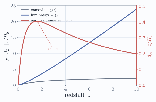
The three distances for Planck ΛCDM, in units of \(c/H_0\). Comoving rises monotonically; luminosity climbs fastest (the \((1+z)\) boost); angular-diameter turns over near \(z\simeq1.6\), the hallmark that distant objects subtend larger angles. From comoving_distance, luminosity_distance, angular_diameter_distance.
Dark energy through \(d_L\). A universe with \(\Lambda\) expanded more slowly in the past, so a source at fixed \(z\) sits farther away and appears fainter — the acceleration signal. Cosmic reproduces Baumann's Figure 2.6 by differing only in the species list:
julia> c_matter = cosmology(Ω_c = 1 - Ω_b(c) - Ω_γ(c) - Ω_ν(c));  # same, but Ω_Λ ≈ 0

julia> luminosity_distance(c, 4.0)         # ΛCDM: a supernova at z = 4, in Mpc
36658.9

julia> luminosity_distance(c_matter, 4.0)  # matter-only: the same supernova
24492.0
Dark energy pushes the \(z=4\) supernova about 50% farther away — and so makes it fainter. That is precisely the surprise the 1998 supernova surveys found, and how they discovered the acceleration of the universe.
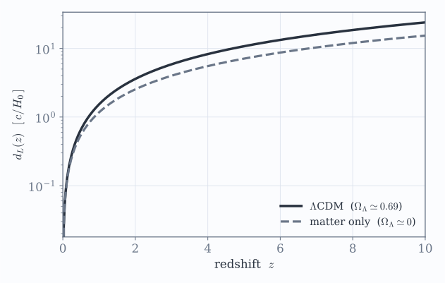
Luminosity distance for ΛCDM versus a flat matter-only universe (Baumann Fig. 2.6). At fixed redshift, dark energy pushes sources farther away and fainter — the effect the 1998 supernova surveys detected.
Flat, open, and closed — with Cosmic.jl. This is where the \(S_k(\chi)\) of Part 1 earns its keep. Handing Cosmic a non-zero \(\Omega_k\) switches \(S_k\) between \(\sin\), \(\chi\) and \(\sinh\), and the angular-diameter distance bends accordingly. Building three matter+curvature universes (closing \(\Omega_\Lambda\approx0\)):
julia> mk(Ωk) = cosmology(Ω_c = 1 - Ω_b(c) - Ω_γ(c) - Ω_ν(c) - Ωk, Ω_k = Ωk);

julia> c_flat, c_open, c_close = mk(0.0), mk(0.7), mk(-0.3);   # k = 0, -1, +1

julia> Ω_k(c_flat), Ω_k(c_open), Ω_k(c_close)
(0.0, 0.7, -0.3)

julia> angular_diameter_distance(c_flat, 3.0)    # flat: a galaxy at z = 3, in Mpc
1108.6

julia> angular_diameter_distance(c_open, 3.0)    # open: the same galaxy, defocused
1580.2

julia> angular_diameter_distance(c_close, 3.0)   # closed: the same galaxy, focused
1000.7
Same galaxy, same redshift, three different-looking answers: curvature alone moves \(d_A\) by 50% either way. Open space defocuses light, so the galaxy looks farther and smaller than it would in flat space; closed space focuses it, so it looks closer and bigger.
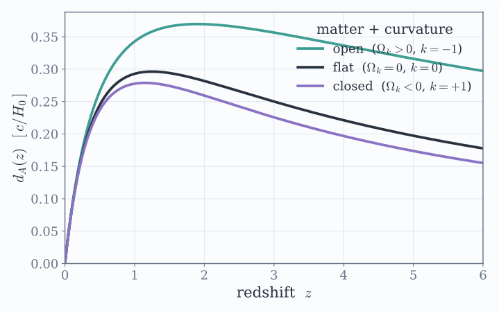
Angular-diameter distance for open (\(k=-1\), \(\sinh\)), flat (\(k=0\)) and closed (\(k=+1\), \(\sin\)) matter universes — all computed by Cosmic.jl from \(\Omega_k\). Open geometry defocuses light so objects look smaller (larger \(d_A\)); closed geometry focuses it so they look bigger (smaller \(d_A\)). It is exactly this sensitivity of \(d_A\) to curvature that lets the CMB measure \(\Omega_k\) to sub-percent precision.
Where we are
We now know how the universe looks: redshift converts scale factor into observation, and three distinct distances translate brightness and angular size into physics — with curvature visibly reshaping them. But we still have not said what drives \(a(t)\). That is Part 3 — Dynamics, where matter and energy enter through the Friedmann equations.