
The Expanding Universe III — Dynamics
Part 3 of five. So far (a(t)) has been an unknown we carried around. Now we make it obey a law — Einstein's equation, fed the contents of the universe — and derive the Friedmann equations and their exact solutions.
In Part 1 symmetry fixed the shape of spacetime; in Part 2 we watched light move on it. Both left \(a(t)\) undetermined. The missing law is the Einstein equation
\[ G_{\mu\nu} = \frac{8\pi G}{c^4}\,T_{\mu\nu} ,\]with \(G_{\mu\nu}\) the curvature and \(T_{\mu\nu}\) the matter content. Plan: constrain \(T_{\mu\nu}\) by symmetry, compute \(G_{\mu\nu}\) for RW, set them equal, solve.
What matter can be: perfect fluids
Homogeneity and isotropy constrain the matter as tightly as they did the geometry. Decompose \(T_{\mu\nu}\) into a scalar \(T_{00}\), vectors \(T_{0i}\), and a tensor \(T_{ij}\). Isotropy forbids a preferred direction, so the mean of any 3-vector vanishes: \(T_{0i}=0\). Isotropy also forces the 3-tensor \(T_{ij}\) to be proportional to the spatial metric, \(T_{ij}\propto g_{ij}\), and homogeneity makes the coefficient a function of time only. Hence
\[ T_{00}=\rho(t)c^2 , \quad T_{0i}=0 , \quad T_{ij}=P(t)\,g_{ij} \;\Longrightarrow\; T^\mu{}_\nu=\mathrm{diag}(-\rho c^2, P, P, P) .\]This is a perfect fluid, and in covariant form
\[ T_{\mu\nu} = \left(\rho+\frac{P}{c^2}\right)U_\mu U_\nu + P\,g_{\mu\nu} .\]Two functions of time: energy density \(\rho c^2\) and pressure \(P\).
Continuity — deriving how \(\rho\) evolves
Energy–momentum conservation is \(\nabla_\mu T^\mu{}_\nu=0\). Unpacking the covariant derivative with the FRW Christoffels (Part 2), the \(\nu=0\) component gives
\[ \partial_\mu T^\mu{}_0 + \Gamma^\mu_{\mu\lambda}T^\lambda{}_0 - \Gamma^\lambda_{\mu 0}T^\mu{}_\lambda = 0 . \]With \(T^0{}_0=-\rho c^2\), \(T^i{}_j=P\delta^i_j\), and \(\Gamma^i_{0j}=c^{-1}(\dot a/a)\delta^i_j\) (three of them), this becomes the continuity equation:
\[ \boxed{\;\dot\rho + 3\frac{\dot a}{a}\left(\rho+\frac{P}{c^2}\right)=0.\;}\]The \(3(\dot a/a)\) is dilution by the growing volume (\(V\propto a^3\)); the pressure term is the work the fluid does as space expands. (The same logic applied to a conserved number current \(\nabla_\mu N^\mu=0\) gives \(n\propto a^{-3}\) — pure volume dilution.)
Equation of state and the density scalings
Close the system with an equation of state \(w\equiv P/\rho c^2\). For constant \(w\), the continuity equation is separable:
\[ \frac{\dot\rho}{\rho} = -3(1+w)\frac{\dot a}{a} \;\Longrightarrow\; \boxed{\;\rho\propto a^{-3(1+w)}.\;}\]
The Friedmann equations
Computing \(G_{\mu\nu}\) for the RW metric is a Christoffel grind (Baumann does it once "to appreciate computer algebra"). The nonzero Ricci pieces are \(R_{00}=-3\ddot a/(c^2a)\) and \(R_{ij}=c^{-2}[\ddot a/a+2(\dot a/a)^2+2kc^2/(a^2R_0^2)]g_{ij}\), giving the Einstein tensor components
\[ G^0{}_0 = -\frac{3}{c^2}\!\left[\left(\frac{\dot a}{a}\right)^2+\frac{kc^2}{a^2R_0^2}\right], \qquad G^i{}_j = -\frac{1}{c^2}\!\left[2\frac{\ddot a}{a}+\left(\frac{\dot a}{a}\right)^2+\frac{kc^2}{a^2R_0^2}\right]\delta^i_j .\]Setting \(G^0{}_0=(8\pi G/c^4)T^0{}_0=-(8\pi G/c^2)\rho\) gives the (first) Friedmann equation:
\[ \boxed{\;\left(\frac{\dot a}{a}\right)^2 = \frac{8\pi G}{3}\rho - \frac{kc^2}{a^2R_0^2}.\;}\]The spatial component \(G^i{}_j=(8\pi G/c^4)T^i{}_j\) gives the second, the Raychaudhuri equation:
\[ \boxed{\;\frac{\ddot a}{a} = -\frac{4\pi G}{3}\left(\rho+\frac{3P}{c^2}\right).\;}\]The first says the expansion rate is sourced by the total density, offset by curvature; the second says gravity decelerates the expansion whenever \(\rho+3P/c^2>0\) — which is why ordinary matter demands a Big Bang, and why acceleration needs something with \(w<-\tfrac13\).
The master equation
Measure densities against the critical density \(\rho_{c,0}=3H_0^2/8\pi G\), and define \(\Omega_i\equiv\rho_{i,0}/\rho_{c,0}\). Dividing the Friedmann equation by \(H_0^2\) and inserting the scalings turns it into the equation Cosmic.jl solves for every calculation in this course:
\[ \boxed{\;\frac{H^2}{H_0^2} = \Omega_r a^{-4} + \Omega_m a^{-3} + \Omega_k a^{-2} + \Omega_\Lambda \equiv E(a)^2,\;}\]with curvature "density" \(\Omega_k\equiv-kc^2/(R_0H_0)^2\). At \(a=1\) this is the closure relation \(\Omega_r+\Omega_m+\Omega_\Lambda+\Omega_k=1\). Measuring these numbers is the central task of observational cosmology — and it is exactly the species list you hand cosmology().
Exact solutions
Single component (flat). With one fluid, \(\dot a/a=H_0\sqrt{\Omega_i}\,a^{-3(1+w)/2}\). Separating and integrating \(\int a^{3(1+w)/2-1}\mathrm d a\propto t\),
\[ a(t)\propto\begin{cases} t^{1/2} & \text{radiation }(w=\tfrac13)\\ t^{2/3} & \text{matter }(w=0)\\ e^{H_0\sqrt{\Omega_\Lambda}\,t} & \Lambda\ (w=-1)\end{cases}\]These three limiting cases have names, and they come up again and again, so it is worth knowing what each one is in plain terms:
Because the densities scale so differently, our universe is dominated by one component at a time — radiation, then matter, then dark energy:
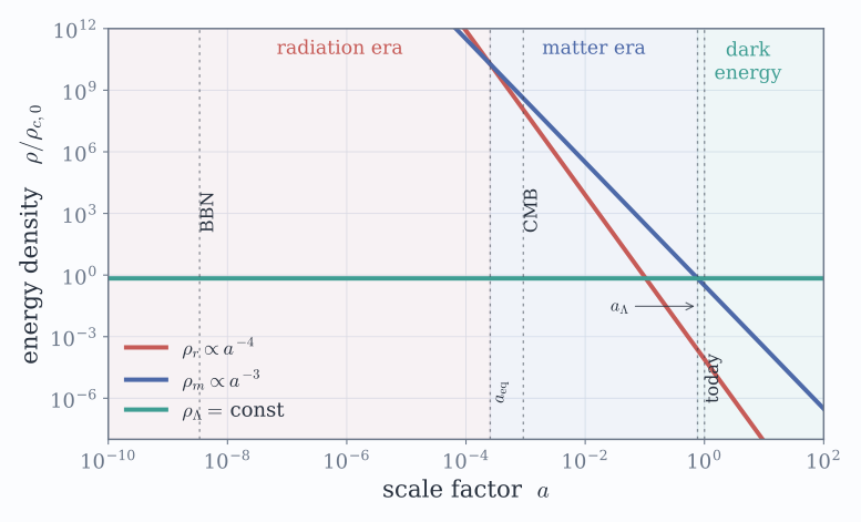
The energy budget through cosmic history (Baumann Fig. 2.10), from the Cosmic.jl density parameters. Radiation (\(a^{-4}\)) dominates before \(a_{\rm eq}\); matter (\(a^{-3}\)) rules from equality until \(a_\Lambda\); the cosmological constant inherits the universe near today. BBN and the CMB (last scattering) sit deep in the radiation and matter eras respectively.
Feeding the full species list to Cosmic.jl and integrating the Friedmann equation reproduces these power laws as the limiting slopes of one smooth curve:
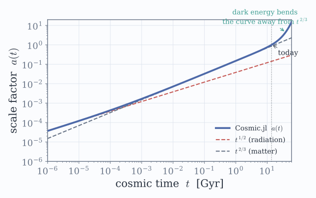
The Cosmic.jl expansion history \(a(t)\) (solid) against the single-fluid asymptotes \(t^{1/2}\) (radiation) and \(t^{2/3}\) (matter). The real universe interpolates smoothly, each component handing off to the next, and the analytic limits fall right on the numerical curve.
Matter + curvature: the fate of the universe. Before dark energy, the destiny of the cosmos hinged on curvature. Working in conformal time, the matter+curvature Friedmann equation \(2\,\mathrm d\widetilde\mathcal H/\mathrm d\theta+\widetilde\mathcal H^2+k=0\) (with \(\theta\equiv c\eta/R_0\)) integrates to the exact parametric solution
\[ a(\theta)=A\begin{cases}\sin^2(\theta/2) & k=+1\\ \theta^2 & k=0\\ \sinh^2(\theta/2) & k=-1\end{cases}, \qquad t(\theta)=\frac{R_0A}{2c}\begin{cases}\theta-\sin\theta\\ \theta^3/3\\ \sinh\theta-\theta\end{cases}\]A closed (\(\Omega_0>1\)) universe reaches a maximum \(a_{\rm max}=\Omega_0/(\Omega_0-1)\) where \(H=0\) and then recollapses to a Big Crunch; an open (\(\Omega_0<1\)) universe expands forever; the flat case is the knife-edge Einstein–de Sitter. Cosmic.jl integrates all three directly from \(\Omega_k\) (the closed branch stops at turnaround, where \(E(a)\to0\)):
julia> mk(Ωk) = cosmology(Ω_c = 1 - Ω_b(c) - Ω_γ(c) - Ω_ν(c) - Ωk, Ω_k = Ωk);

julia> c_flat, c_open, c_close = mk(0.0), mk(0.7), mk(-0.3);   # k = 0, -1, +1

julia> Ω_m(c_close), Ω_k(c_close)     # a closed universe has Ω_m > 1 and Ω_k < 0
(1.2985, -0.3)

julia> a_max = Ω_m(c_close) / abs(Ω_k(c_close))   # it turns around here, where H = 0
4.328

julia> E(c_close, a_max)              # the expansion rate does vanish at turnaround
2.1e-8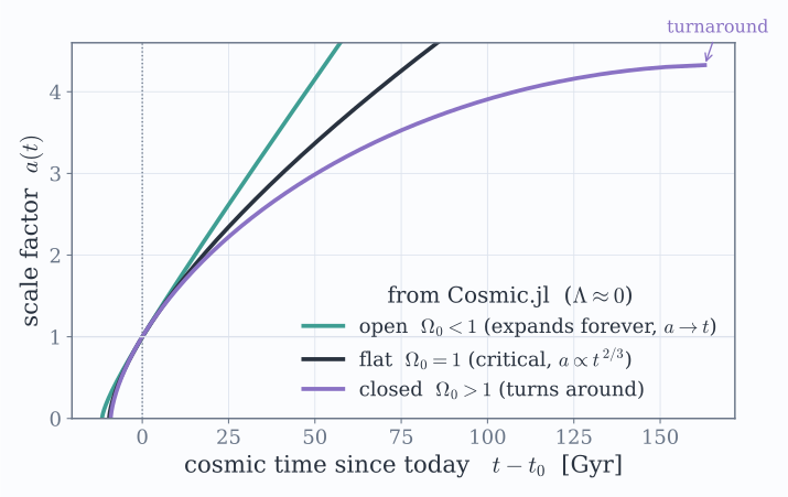
The fate of matter+curvature universes (Baumann Fig. 2.12), computed by Cosmic.jl by integrating \(\dd t = \dd a/(aH_0E(a))\) for each \(\Omega_k\). Open (\(\Omega_0<1\)) expands forever; flat (\(\Omega_0=1\)) coasts to a halt at infinity; closed (\(\Omega_0>1\)) reaches \(a_{\rm max}\) and turns around toward a Big Crunch. Our universe sits astonishingly close to the flat divider — the flatness problem.
Matter + \(\Lambda\): our universe. A flat universe with matter and a cosmological constant has \(H^2/H_0^2=\Omega_m a^{-3}+\Omega_\Lambda\). Unlike the single-fluid and curvature cases above, this one is not solved by a direct power-law ansatz — it needs a substitution, so let's actually do it. Write \(\dot a/a=H_0\sqrt{\Omega_m a^{-3}+\Omega_\Lambda}\) and multiply through by \(a^{3/2}\):
\[ a^{1/2}\dot a = H_0\sqrt{\Omega_m+\Omega_\Lambda a^3} = H_0\sqrt{\Omega_m}\,\sqrt{1+(a/a_\Lambda)^3}, \qquad a_\Lambda\equiv\left(\frac{\Omega_m}{\Omega_\Lambda}\right)^{1/3} .\]The left side is \(\tfrac23\mathrm d(a^{3/2})/\mathrm d t\), which is the tell that \(x\equiv(a/a_\Lambda)^{3/2}\) is the right variable: \(a^{3/2}=a_\Lambda^{3/2}x\), so \(\tfrac23a_\Lambda^{3/2}\dot x=H_0\sqrt{\Omega_m}\sqrt{1+x^2}\). Since \(a_\Lambda^{-3/2}=\sqrt{\Omega_\Lambda/\Omega_m}\), the \(\Omega_m\)'s cancel and this separates cleanly,
\[ \frac{\mathrm d x}{\sqrt{1+x^2}} = \tfrac32\sqrt{\Omega_\Lambda}\,H_0\,\mathrm d t \;\Longrightarrow\; \sinh^{-1}x = \tfrac32\sqrt{\Omega_\Lambda}H_0 t ,\]fixing the integration constant by \(a=0\) (so \(x=0\)) at \(t=0\), the Big Bang. Undoing \(x=(a/a_\Lambda)^{3/2}\) gives the closed form, and setting \(a(t_0)=1\) gives the age:
\[ \boxed{\;a(t)=\left(\frac{\Omega_m}{\Omega_\Lambda}\right)^{1/3}\sinh^{2/3}\!\left(\tfrac32\sqrt{\Omega_\Lambda}\,H_0 t\right)\;}, \qquad t_0=\frac{2}{3\sqrt{\Omega_\Lambda}H_0}\sinh^{-1}\!\sqrt{\frac{\Omega_\Lambda}{\Omega_m}} .\]The two limits confirm it stitches together the two universes we already know. Early on \(a\ll a_\Lambda\) means \(x\ll1\), where \(\sinh^{-1}x\approx x\), so \(a(t)\propto t^{2/3}\) — plain Einstein–de Sitter, matter not yet noticing \(\Lambda\). Late on \(a\gg a_\Lambda\) means \(x\gg1\), where \(\sinh x\approx\tfrac12e^x\), so \(a(t)\propto e^{H_0\sqrt{\Omega_\Lambda}\,t}\) — de Sitter, matter diluted away and only the constant left. With \(\Omega_m=0.31,\Omega_\Lambda=0.69\) the age comes out \(t_0\approx0.96\,H_0^{-1}\approx14\,\mathrm{Gyr}\) — a universe old enough for its oldest stars, unlike EdS — and matches what Cosmic returns below.
A universe of matter obeying \(\rho+3P/c^2>0\) must have had a singularity — because \(\ddot a<0\) everywhere means \(a(t)\), run back from today's expansion, hit zero. That is the FRW baby version of the Hawking–Penrose theorems.
Verifying with Cosmic.jl
The tightest check of the course: \(E(a)\) is literally the species sum, and the deceleration parameter follows from its slope.
First, that \(E(a)^2\) really is the sum over species — compare it against the textbook two-power form at, say, \(a=0.1\):
julia> a = 0.1;

julia> E(c, a)^2                              # the exact Friedmann sum, Σ ρ_s(a)/ρ_c0
313.3

julia> Ω_r(c)*a^-4 + Ω_m(c)*a^-3 + Ω_de(c)    # the textbook Ω_r a⁻⁴ + Ω_m a⁻³ + Ω_Λ
311.9
They agree to about half a percent, and the small gap is physics, not error: at \(a=0.1\) the massive neutrino is partway between behaving like radiation and like matter, and the clean two-power split can't capture it — a reminder of why Cosmic tracks each species' real \(\rho(a)\).
Next, the deceleration parameter \(q_0=-\ddot a a/\dot a^2\big|_0\), which is negative if the universe accelerates. We can read it straight off the slope of \(E(a)\):
julia> δ = 1e-4;

julia> q0 = -1 - (log(E(c, exp(δ))) - log(E(c, exp(-δ)))) / (2δ)   # from the slope of E(a)
-0.544

julia> 0.5*Ω_m(c) + Ω_r(c) - Ω_de(c)          # the textbook formula ½Ω_m + Ω_r − Ω_Λ
-0.534
Both are negative — our universe is accelerating. Finally, the age problem and its resolution, side by side:
julia> 2/3 * hubble_time(c)      # the Einstein–de Sitter (matter-only) age, in Gyr
9.634

julia> age(c)                    # the real, Λ-included age
13.787
The matter-only universe would be only 9.6 Gyr old — younger than the oldest stars. Dark energy stretches the real age to 13.8 Gyr, comfortably older, exactly as promised.
Where we are
We have the law of motion: the Friedmann equations, the density scalings, and the exact solutions for each era and geometry. Everything is ready for the measured numbers. Part 4 — Our Universe puts them in — the cosmic budget, the age, equality, and the thermal history — Cosmic.jl against the observed values.