feynsage: a Tutorial for Someone Starting QFT

In a first QFT course the calculations arrive in a fixed order. First you learn to take traces of gamma matrices. Then you square an amplitude, average over spins, turn it into a cross section you could compare with an experiment. Loops come later, once the easy things are safe.

feynsage is a SageMath package that does these calculations. This page follows that same order.

Who this is for. You have met the Dirac equation, you have seen a Feynman diagram, you know that a cross section is what an experiment measures. You do not need to have taken a single trace by hand, because we start there.

Everything on this page is real output. Each block was run, the answer captured, then typeset.

Installing it

git clone https://github.com/aburousan/feynsage.git
cd feynsage
./install.sh          # add --test to run the test suite afterwards

The script finds SageMath with FORM, or installs them. Then, inside Sage:

from feynsage import *

Part 1: gamma matrices and traces

What these objects are

The Dirac equation describes a spin one-half particle such as an electron. To write it down you need four matrices, \(\gamma^0,\gamma^1,\gamma^2,\gamma^3\), each one a \(4\times4\) matrix. They are called gamma matrices or Dirac matrices.

You almost never need the matrices themselves. Everything follows from one rule, the anticommutation relation

\[ \gamma^\mu\gamma^\nu + \gamma^\nu\gamma^\mu = 2g^{\mu\nu} \]

Two more pieces of notation. A slash is a momentum contracted with the gammas,

\[ \not p \equiv p_\mu\gamma^\mu \]

and the trace of a matrix is the sum of its diagonal entries, written \(\mathrm{tr}\).

🧠 Defn

Why traces appear at all. This is the part that is usually left unsaid.

An amplitude \(\mathcal M\) for a process with electrons carries spinors \(u(p)\) with gamma matrices between them. What an experiment measures is not \(\mathcal M\) but \(|\mathcal M|^2\), usually averaged over the spins you did not prepare, summed over the spins you did not measure.

Doing that sum over spins uses the identity \(\sum_s u(p)\bar u(p) = \not p + m\). Once you put it in, the spinors are gone, every term becomes a string of gamma matrices with its ends joined. A string of matrices with its ends joined is a trace.

So: spin sum in, trace out. That is why a QFT course spends a week on trace identities before computing anything physical.

Taking traces

In feynsage you declare your momenta with your indices, then write the trace the way the book writes it. FORM does the algebra underneath, you never see it.

p, q = momenta('p q')
mu, nu, rho, sigma_ = lorentz_indices('mu nu rho sigma_')

Start with the simplest one, the trace of the identity matrix. It is a \(4\times4\) matrix, so:

dirac_trace(one())

\[ 4 \]

Two gammas:

dirac_trace(gamma(mu)*gamma(nu))

\[ 4 \, g^{\mu \nu} \]

An odd number of them gives nothing at all:

dirac_trace(gamma(mu)*gamma(nu)*gamma(rho))

\[ 0 \]

Four gammas, the identity that takes half a page by hand:

dirac_trace(gamma(mu)*gamma(nu)*gamma(rho)*gamma(sigma_))

\[ 4 \, g^{\mu \sigma} g^{\nu \rho} - 4 \, g^{\mu \rho} g^{\nu \sigma} + 4 \, g^{\mu \nu} g^{\rho \sigma} \]

Those four results are exactly the trace theorems Peskin and Schroeder collect in equation (5.5) on page 134, which is the box a first course asks you to memorise. Now with momenta in them:

dirac_trace(slash(p)*slash(q))

\[ 4 \, \left(p \cdot q\right) \]

dirac_trace(slash(p)*gamma(mu)*slash(q)*gamma(nu))

\[ 4 \, p^{\nu} q^{\mu} + 4 \, p^{\mu} q^{\nu} - 4 \, \left(p \cdot q\right) g^{\mu \nu} \]

Each of these came back in under three hundredths of a second. The last one is the trace you meet in the first real calculation of the course, which is where we go next.

Part 2: a cross section you could measure

The process

Take the reaction an electron-positron collider actually does:

\[ e^- e^+ \to \mu^- \mu^+ \]

An electron meets a positron, they annihilate into a photon, the photon turns into a muon with an antimuon. It is the standard first calculation because it has exactly one diagram in QED, no complications.

🧠 Defn

\(s\), \(t\) and \(u\), if nobody has defined them yet. Call the incoming momenta \(p_1,p_2\) with the outgoing ones \(p_3,p_4\). Three combinations describe the whole kinematics:

\[ s=(p_1+p_2)^2, \qquad t=(p_1-p_3)^2, \qquad u=(p_1-p_4)^2 \]

\(s\) is the total energy squared in the centre of mass, so \(\sqrt{s}\) is the collider energy. \(t\) with \(u\) carry the scattering angle. feynsage will print answers in these variables.

Set the process up. We ask for pure QED, so only the photon is exchanged, with the electron and muon masses set to zero since the collider energy is far above both:

qed = QED()
P = process('e- e+ -> mu- mu+', model=qed, massless=['e', 'mu'])
len(P.diagrams)

\[ 1 \]

One diagram, as expected.

The squared amplitude

P.squared()

\[ \frac{2 \, \left(e^{4} t^{2} + e^{4} u^{2}\right)}{s^{2}} \]

That is \(|\mathcal M|^2\), already averaged over the two initial spins, summed over the final ones. Written tidily,

\[ \overline{|\mathcal M|^2} = \frac{2e^4\left(t^2+u^2\right)}{s^2} \]

feynsage built the diagram, put in the spin sums, took the traces of Part 1, contracted the indices, then averaged, in two hundredths of a second. Peskin works the same process through section 5.1 with the masses kept, writing the answer in the energy with the angle instead of in \(t\) with \(u\).

Turning it into a cross section

A squared amplitude is not yet something you can measure. You must divide by the flux, integrate over the directions the muons can come out in. The useful quantity is the differential cross section \(\mathrm d\sigma/\mathrm d\cos\theta\), which says how much of the scattering goes into each angle, with \(\theta\) the angle between the incoming electron with the outgoing muon.

P.dsigma_dcos()

\[ \frac{e^{4} \cos\theta^{2} + e^{4}}{32 \, \pi \sqrt{s}^{2}} \]

Read the shape off it: the answer is proportional to \(1+\cos^2\theta\). Using \(e^2 = 4\pi\alpha\) this is

\[ \frac{\mathrm d\sigma}{\mathrm d\cos\theta} = \frac{\pi\alpha^2}{2s}\left(1+\cos^2\theta\right) \]

This is Peskin's equation (5.14) on page 137, written there as \(\mathrm d\sigma/\mathrm d\Omega = (\alpha^2/4E_{\rm cm}^2)(1+\cos^2\theta)\). The two agree: the solid angle brings a factor \(2\pi\), since nothing depends on the azimuth, with \(E_{\rm cm}^2 = s\).

More muons come out along the beam than across it, in that particular shape. It is a real prediction that experiments have confirmed many times.

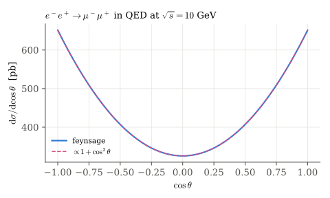
The angular distribution at \(\sqrt{s}=10\) GeV, in picobarns. The solid curve is what feynsage computed, the dashed one is the shape \(1+\cos^2\theta\) normalised at the middle. They lie on top of each other.

Now integrate over all angles to get one number:

P.sigma(sqrt_s=10, unit='pb')

\[ 868.5447687569202 \]

🧠 Defn

What a picobarn is. Cross sections have units of area, because the classical picture is the size of the target. The unit is the barn, \(10^{-28}\,\mathrm{m}^2\), which is enormous by nuclear standards, named from "as big as a barn door". A picobarn is \(10^{-12}\) of that.

So the answer says: at a collider running at \(\sqrt{s}=10\) GeV, the effective target area for making a muon pair is about 869 pb.

Check it against the textbook. In the high-energy limit the total cross section is

\[ \sigma = \frac{4\pi\alpha^2}{3s} \]

which is the formula on Peskin page 137, where the text notes that dimensional analysis fixes everything except the factor \(4\pi/3\). At \(\sqrt s = 10\) GeV it gives \(868.546\) pb against feynsage's \(868.545\) pb. The leftover difference, about one part in a million, is the constant used to convert \(\mathrm{GeV}^{-2}\) into picobarns.

That is a complete calculation, from naming a reaction to a number with units, in four lines.

Part 3: loops, when you get there

Everything above was tree level, meaning the diagram has no closed loops in it. Later in the course the diagrams grow a loop, with a momentum running round it that is not fixed by the incoming particles, so you must integrate over all of it:

\[ \int \frac{\mathrm d^4\ell}{(2\pi)^4}\;\frac{1}{(\ell^2-m^2)\left((\ell+p)^2-m^2\right)} \]

These integrals are the hard part of QFT. Many of them come out infinite, which is what renormalisation exists to handle.

feynsage knows the standard ones by name. The simplest, one propagator in a circle, is called the tadpole:

A0('m')

\[ m^{2} \left(\frac{1}{\epsilon} + \log\left(\frac{\mu^{2}}{m^{2}}\right) + 1\right) \]

The \(1/\epsilon\) is the infinity, held in a form you can cancel later. \(\mu\) is a reference energy that the method needs. With two propagators you get the bubble, which depends on the momentum \(s\) flowing through:

s = var('s')
B0(s, 'm', 'm')

\[ \frac{1}{\epsilon} + \Lambda(s; m, m) + \log\left(\frac{\mu^{2}}{m^{2}}\right) + 2 \]

\(\Lambda\), printed as DiscB, holds all the dependence on \(s\).

Why the bubble has an imaginary part

Here is the one loop result worth seeing even on a first pass. Take the finite part of the bubble, evaluate it along the real \(s\) axis:

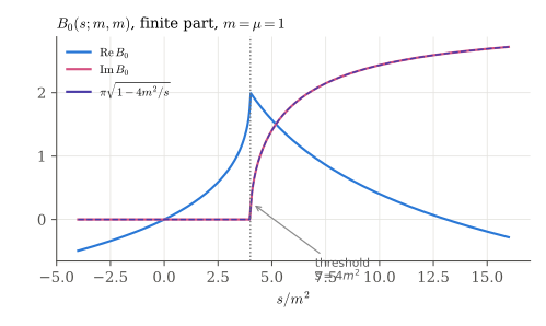
The finite part of \(B_0(s;m,m)\) with \(m=\mu=1\). Below \(s=4m^2\) it is real. At \(s=4m^2\) an imaginary part switches on, which is exactly the energy needed to make the two particles inside the loop real instead of virtual. The dashed line is \(\pi\sqrt{1-4m^2/s}\), sitting on what feynsage computed.

The threshold is the optical theorem: the imaginary part of a loop is the rate for actually producing what is inside it, so it must be zero until there is enough energy. Checked at four points:

\(s/m^2\)	feynsage	\(\pi\sqrt{1-4m^2/s}\)
5	1.4049629462081452	1.4049629462081452
9	2.3416049103469088	2.3416049103469088
16	2.720699046351327	2.7206990463513265
100	3.078119592388474	3.0781195923884734

The conventions, before you compare with a book

🧠 Defn

The arguments are masses, not masses squared. A0('m') means a particle of mass \(m\), following Package-X. So A0('m^2') describes a particle of mass \(m^2\) and returns \(m^4(\dots)\). If a power looks wrong, check this first. (The inert functions PaVeA0, PaVeB0 and friends are the exception: those take squared masses.)

The dimension is \(d=4-2\epsilon\). Loop integrals are normalised as

\[ \mu^{2\epsilon}e^{\epsilon\gamma_E}\frac{1}{i\pi^{d/2}}\int \mathrm d^d\ell \]

so the \(\gamma_E\) with the \(\log 4\pi\) are absorbed. You get the \(\overline{\rm MS}\) answer.

Peskin uses \(d=4-\epsilon\). His poles are \(2/\epsilon\) where feynsage writes \(1/\epsilon\). Compare the two directly, you find a factor of two that is not physics.

The metric is \((+,-,-,-)\), with the propagator denominator \(q^2-m^2+i0\).

Where to go next

feynsage goes a long way past this page: tensor reduction of loop integrals, integral families, IBP reduction with symmetries found by itself, master integrals, Mellin-Barnes, sector decomposition, differential equations, diagrams generated from a model the way FeynArts does it.

• The repository with the full reference: github.com/aburousan/feynsage

• A longer tutorial ships inside it at docs/tutorial/feynsage_tutorial.pdf

• docs/dirac_algebra.md if traces are what you came for

• Many functions explain themselves. Pass explain=True to the one-loop functions such as A0, or call info(f) on a function, to have it print what the output means.

One honest word on scale. feynsage is built for small and medium problems, where every step stays exact, can be checked, explains itself. For very large reductions with millions of equations, Kira with FIRE are the right tools.

Go Back