
- The question nobody asks in the first lecture
- One line of algebra is the whole idea
- Doing it properly: one heavy scalar
- What "matching" means
- The real one: Fermi and beta decay
- How wrong are you? The part that makes it a science
- Counting dimensions, which turns out to be the whole skill
- "Non-renormalisable" is not an insult
- A worked example: hydrogen, without bottom quarks
- Scalar QED, which you have already met
- The QED one: light that scatters off light
- What this post did not tell you
- Exercises
- Where to read more
Effective Field Theory, Starting From the Propagator You Just Learned
You are a few weeks into a first course on quantum field theory. You know what a propagator is. You can write \(\dfrac{i}{p^2-m^2+i\varepsilon}\) for a scalar without looking it up, you have met the photon and electron propagators in QED, you can read a tree diagram.
That is enough. With it you can understand what an effective field theory is, which is one of the ideas that working physicists use every day.
Here is the whole thing in one sentence. You cannot use a particle you do not have the energy to make, so it should be possible to write down a theory without it. Everything below is that sentence, done carefully.
The question nobody asks in the first lecture
Physics has a peculiar piece of good luck built into it.
Nobody knows the final theory. There may be new particles at energies we cannot reach, there is certainly something going on at the Planck scale where gravity becomes quantum. Yet a chemist predicts a reaction rate without any of it. A hydrogen atom was solved in 1926 by people who had never heard of a quark.
Why should that work? If physics at short distances is unknown, why is physics at long distances not also unknown?
One line of algebra is the whole idea
Take the propagator you already know, for a particle of mass \(M\) carrying momentum \(q\):
\[ \frac{i}{q^2 - M^2}. \]Now suppose \(M\) is huge. The particle is far too heavy to produce in your experiment, so every momentum in your problem is small: \(|q^2| \ll M^2\). (The absolute value matters. The momentum through an internal line can be negative when the particles are deflected rather than annihilated, so the condition is on the size of \(q^2\), not on its sign.) Look at what the propagator becomes. Pull out the \(-M^2\):
\[ \frac{1}{q^2-M^2} = \frac{-1}{M^2}\cdot\frac{1}{1 - q^2/M^2} = -\frac{1}{M^2}\left(1 + \frac{q^2}{M^2} + \frac{q^4}{M^4} + \cdots\right), \]using nothing more than \(\dfrac{1}{1-x} = 1 + x + x^2 + \cdots\) for small \(x\).
Read the right-hand side slowly, because it is the entire subject.
The leading term, \(-1/M^2\), has no \(q\) in it at all. A propagator that does not depend on momentum is not a particle travelling anywhere. In position space, momentum dependence is what lets a disturbance move from one place to another, so a constant means the interaction happens at a single point. The heavy particle has stopped being a thing that propagates. It has become a contact interaction.
The rest of the series, in powers of \(q^2/M^2\), are the corrections that remember the particle was really there.
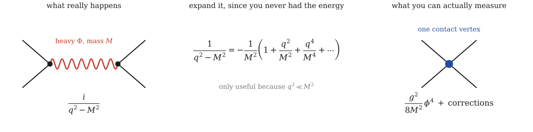
At energies far below \(M\), the exchanged heavy line shrinks to a point. The internal line is still really there, but nothing you can measure at low energy can resolve it, so a single contact vertex reproduces every number you can check.
Doing it properly: one heavy scalar
Let us do the calculation rather than wave at it. Take a light scalar \(\phi\) with mass \(m\) and a heavy one \(\Phi\) with mass \(M \gg m\), coupled in the simplest way that is allowed:
\[ \mathcal L = \tfrac12(\partial\phi)^2 - \tfrac12 m^2\phi^2 + \tfrac12(\partial\Phi)^2 - \tfrac12 M^2\Phi^2 - \frac{g}{2}\,\Phi\,\phi^2 . \]The last term lets one heavy particle turn into two light ones. Its Feynman rule is a vertex joining one \(\Phi\) line to two \(\phi\) lines, worth \(-ig\). (The \(\tfrac12\) in the Lagrangian cancels against the two ways of attaching the two identical \(\phi\) legs, which is the usual business with symmetry factors.)
Now scatter two light particles off each other, \(\phi\phi\to\phi\phi\). At tree level the only thing that can happen is that the two incoming particles make a virtual \(\Phi\), which then turns back into two.
How many ways can that happen? Label the four external lines \(1,2,3,4\). The heavy line has to separate them into two pairs, with two legs at each end. There are exactly three ways to split four objects into two pairs:
\[ \underbrace{(12)(34)}_{s\ \text{channel}}, \qquad \underbrace{(13)(24)}_{t\ \text{channel}}, \qquad \underbrace{(14)(23)}_{u\ \text{channel}}. \]Each bracket is one vertex: the two legs inside it meet there, with the heavy line running between the two brackets. Taking \(1,2\) as the incoming particles with \(3,4\) outgoing, the first pairing has both incoming particles meeting at the same vertex, while the other two have one incoming particle meeting one outgoing particle. Those are the \(s\), \(t\) and \(u\) channels, defined next. (It is the same "three pairings of four things" that turns up in Wick's theorem, for the same combinatorial reason.)
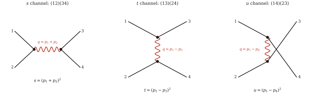
The same three pairings, drawn. In the \(s\) channel the two incoming particles meet first, so the heavy line (red) carries everything they brought in. In the \(t\) and \(u\) channels the heavy line is handed across, carrying only the difference between an incoming and an outgoing momentum. The \(u\) channel is the \(t\) channel with the two outgoing legs swapped, which is why its lines cross.
So the amplitude is the sum of three diagrams, each one made of two vertices with one heavy propagator between them:
\[ \mathcal M = \underbrace{(-ig)}_{\text{vertex}}\underbrace{\frac{i}{s-M^2}}_{\text{propagator}}\underbrace{(-ig)}_{\text{vertex}} \;+\; (s\to t) \;+\; (s\to u) = (-ig)^2\left[\frac{i}{s-M^2} + \frac{i}{t-M^2} + \frac{i}{u-M^2}\right]. \]Now set the energies low. Every one of \(s\), \(t\), \(u\) is far smaller than \(M^2\), so in each denominator the \(M^2\) wins outright and \(s-M^2 \to -M^2\). All three terms become the same thing:
\[ \frac{i}{-M^2} + \frac{i}{-M^2} + \frac{i}{-M^2} = -\frac{3i}{M^2}. \]For the prefactor, \((-ig)^2 = (-i)^2g^2 = -g^2\). Multiplying the two pieces:
\[ \mathcal M \;\longrightarrow\; (-g^2)\times\left(-\frac{3i}{M^2}\right) = \frac{3ig^2}{M^2}. \]A constant. No dependence on the angle, no dependence on the energy. That is the signature of a contact interaction: momentum dependence is what tells you something travelled a distance, so an amplitude with no momentum in it describes particles meeting at a point. (In position space the statement is that the Fourier transform of a constant is a delta function, which is a "do it here, at one place" instruction.)
Now build the theory without the heavy particle. Take \(\phi\) alone, with an interaction term \(c\,\phi^4\) in the Lagrangian. What is its four-point vertex?
The Feynman rule for a vertex is \(i\) times the coefficient in \(\mathcal L\), times the number of ways of attaching the external lines to the fields in the operator. Here \(\phi^4\) has four identical fields, while we have four external lines to attach. The first line can go to any of the 4 fields, the second to any of the remaining 3, the third to either of the remaining 2, the last to the 1 left over:
\[ 4\times3\times2\times1 = 4! = 24 . \]So the vertex is \(i\,c\cdot 24 = 24\,i\,c\). (This is exactly why couplings are conventionally written with a \(1/4!\) in front. Writing the interaction as \(-\frac{\lambda}{4!}\phi^4\) makes the vertex \(i\cdot(-\lambda/4!)\cdot 4! = -i\lambda\), with the 24 cancelling against the \(4!\) that was put there for exactly that purpose.)
Match the two. Demand that the effective theory give the same amplitude as the full one:
\[ 24\,i\,c = \frac{3ig^2}{M^2}. \]The \(i\) cancels on both sides. Dividing by 24:
\[ c = \frac{3g^2}{24\,M^2} \qquad\Longrightarrow\qquad \boxed{\;c = \frac{g^2}{8M^2}.\;} \]That is an effective field theory. Below the energy needed to make a \(\Phi\), the theory with a heavy scalar and the theory without one give the same answer for this process, provided you choose \(c\) to be \(g^2/8M^2\).
What "matching" means
The step where you forced the two theories to agree has a name: matching.
The recipe is always the same. Compute something in the theory you believe (the "full" theory, with the heavy particle). Compute the same thing in the theory you want to use (the "effective" theory, without it). Choose the coefficients in the effective theory so the answers agree. From then on use the effective theory, which is simpler.
Two things are worth noticing.
The coefficient remembers. \(c = g^2/8M^2\) carries \(g\) and \(M\) in it, the two things the low-energy theory supposedly knows nothing about. The heavy physics did not vanish. It was compressed into one number.
It works in reverse. Suppose you did not know about \(\Phi\) at all. You measure \(\phi\phi\) scattering, find a contact interaction of strength \(c\), then write it down. You have a perfectly good theory. What you have measured is \(c\), full stop. Reading it as \(g^2/8M^2\) is already assuming this particular heavy scalar: a different mediator, or a different interaction, can produce the same \(c\). So you cannot tell from \(c\) alone whether it came from a heavy scalar with some \(g\) and \(M\), from a different \(g'\) and \(M'\) with the same ratio, or from something else entirely. That is not a failure. It is exactly as much as your experiment is entitled to know.
The real one: Fermi and beta decay
Now the example that actually happened, which uses the QED-style propagator you know rather than a made-up scalar.
A neutron decays. In the real theory this happens because a \(d\) quark emits a \(W\) boson, which turns into an electron plus an antineutrino. The \(W\) propagator is the massive vector one, with \(m_W = 80.4\) GeV. The energy released in the decay is under \(1.3\) MeV.
So \(q^2/m_W^2 \sim 10^{-10}\). The heavy line shrinks to a point, exactly as above, leaving four fermion lines meeting at one place:
\[ \frac{g^2}{8}\,\frac{1}{q^2-m_W^2}\;\longrightarrow\;-\frac{g^2}{8m_W^2} \;\equiv\; -\frac{G_F}{\sqrt2}. \]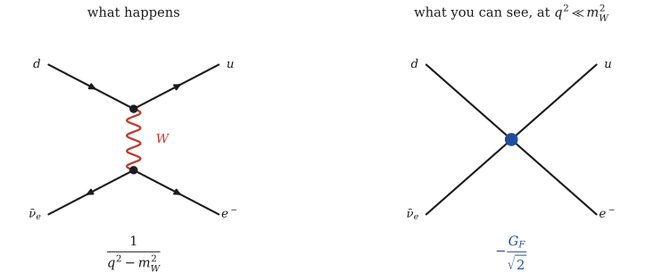
Beta decay at the quark level. On the left, what the Standard Model says happens: a \(d\) quark turns into a \(u\), emitting a \(W\) that becomes the electron with its antineutrino. On the right, what an experiment at MeV energies can resolve: four lines meeting at a point, with one number attached.
Fermi wrote down a four-fermion contact interaction of this kind in 1933. (The particular left-handed structure the Standard Model produces came later, with Feynman and Gell-Mann in 1958.) The \(W\) boson was not found until 1983, fifty years after Fermi. He did not need it, because at the energies of beta decay it is invisible in exactly the sense above: present but unresolvable.
Real neutron decay brings in more than the diagram above, since the neutron is made of quarks that are themselves bound together, plus a quark-mixing factor. None of that changes the point: whatever else is going on, the \(W\) line has shrunk to a point.
How wrong are you? The part that makes it a science
Anyone can say "ignore the heavy stuff". What makes this a method rather than an excuse is that you can say by how much you are wrong, before anyone measures anything.
Go back to the expansion. The corrections come in powers of \(q^2/M^2\), so if your experiment runs at energy \(E\), the error you make by keeping only the contact term is of order \((E/M)^2\). Keep one more term and the error drops to \((E/M)^4\). And so on.
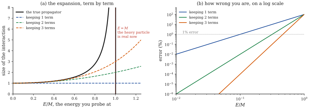
(a) The true propagator against the first few terms of its expansion. (b) The same thing as an error, on log axes, where the lines have slopes 2, 4 and 6: every extra term you keep buys two more powers of \(E/M\). Both panels end at \(E=M\), where the series stops converging because you now have enough energy to make the particle for real.
In numbers, keeping \(N\) terms leaves a relative error of about \(|q^2/M^2|^N\), so at one tenth of the heavy mass:
| terms kept | error at \(E/M = 0.1\) |
|---|---|
| 1 (just the contact term) | 1% |
| 2 | 0.01% |
| 3 | 0.0001% |
Read that table narrowly. It is the error from cutting off this momentum expansion, nothing else. Quantum corrections, other operators you may have forgotten, or an accidentally large coefficient are separate worries that have to be estimated on their own.
For neutron decay the momentum through the \(W\) is at most of order an MeV, so
\[ \frac{|q^2|}{m_W^2} \lesssim \frac{(1.3\ \mathrm{MeV})^2}{(80.4\ \mathrm{GeV})^2} \approx 2.6\times10^{-10}. \]Ten decimal places. Nobody is ever going to see that particular correction.
Be careful about what that sentence claims, though. It is a statement about one correction, the one from having shrunk the \(W\) line to a point. Precision predictions for beta decay need electromagnetic corrections, recoil, nuclear structure and more, all of which are far larger. Shrinking the \(W\) is the one thing you may stop worrying about.
Counting dimensions, which turns out to be the whole skill
Before the next step you need one tool, which costs five minutes to learn. It is the thing that lets you guess the size of an effect without computing a single diagram.
Work in units where \(\hbar = c = 1\), so everything is a power of mass. Two facts set it all up.
Fact one: the action is dimensionless. \(S = \int \mathrm d^4x\,\mathcal L\) appears in \(e^{iS}\), so it cannot carry units. Since \([\mathrm d^4x] = -4\), this forces
\[ [\mathcal L] = 4. \]Fact two: the kinetic term fixes the field. Every scalar Lagrangian starts with \(\tfrac12(\partial\phi)^2\), which must have dimension 4. A derivative carries dimension 1, so \(2 + 2[\phi] = 4\), giving
\[ [\phi] = 1. \](In \(d\) dimensions the same argument gives \([\phi] = \tfrac{d-2}{2}\). For a fermion the kinetic term is \(\bar\psi\,\partial\!\!\!/\,\psi\) with one derivative rather than two, so \([\psi] = \tfrac32\).)
Everything else follows by making each term in \(\mathcal L\) add up to 4.
Show solution
\(m^2\phi^2\): the fields give \(2\times1 = 2\), so \([m^2] = 2\). Good, it is a mass squared.
\(\lambda\phi^4\): the fields give \(4\), so \([\lambda] = 0\). The quartic coupling is a pure number. This is why \(\phi^4\) theory is special in four dimensions.
\(\tau\phi^6\): the fields give \(6\), so \([\tau] = -2\). Negative. It has to be built as \(1/(\text{some mass})^2\).
That last line is the interesting one. A coupling with negative dimension cannot be a pure number. It must contain a mass, hidden somewhere, whether or not you know what that mass is.
Show solution
So \(G_F\) must be \(1/(\text{mass})^2\). The measured value is \(G_F = 1.166\times10^{-5}\ \mathrm{GeV}^{-2}\), which is indeed an inverse mass squared, corresponding to a mass of about \(\sqrt{1/G_F} = 293\) GeV.
Fermi had that number in 1933. Read it as a prediction and it says: somewhere near a few hundred GeV, there is something. The \(W\) turned up at 80 GeV.
Show solution
Then \([c] = [g^2/M^2] = 2-2 = 0\), so the contact term \(c\,\phi^4\) is the marginal kind, like any ordinary \(\phi^4\) coupling. Integrating out the heavy scalar did not by itself produce a "non-renormalisable" interaction at leading order.
The derivative correction is where that happens. Its coefficient is \(g^2/8M^4\), of dimension \(2-4 = -2\), multiplying the operator \(\phi^2\Box\phi^2\) of dimension \(1+1+2+1+1 = 6\). Together: \(-2+6 = 4\), as required.
There is a pattern here worth keeping, as long as you keep its scope with it. In this expansion, every extra factor of \(1/M^2\) arrives with two more derivatives, because the series was in \(q^2/M^2\) while each \(q\) becomes a \(\partial\) in position space.
It is not a universal law. An operator can climb in dimension by collecting more fields instead of more derivatives, which is exactly what \(\phi^6\) does in Worked example 1: dimension 6, coefficient \(1/M^2\), not a derivative in sight.
Show solution
Dimension 2. Two fields, no derivatives: \(\phi^2\). Its coefficient has dimension 2, so it is a mass squared. This is the mass term.
Dimension 4. Either four fields, \(\phi^4\), or two fields with two derivatives, \((\partial_\mu\phi)(\partial^\mu\phi)\). The second is the kinetic term, whose coefficient is fixed at \(\tfrac12\) by insisting the field be normalised the usual way. The first has a dimensionless coefficient.
Dimension 6. Now the possibilities open up. Six fields with no derivatives, \(\phi^6\). Four fields with two derivatives, \(\phi^2(\partial\phi)^2\). Two fields with four derivatives, \((\Box\phi)^2\). Each coefficient has dimension \(-2\), so each is some number over \(M^2\).
The pattern to take away is that the list at each dimension is finite. That is what makes an effective theory predictive rather than a licence to write anything: you cannot be surprised at dimension 6 by an operator nobody thought of, because you can enumerate them all in an afternoon.
"Non-renormalisable" is not an insult
Somewhere in your course you will meet a rule that goes roughly: theories with couplings of negative mass dimension are non-renormalisable, therefore bad.
You have just built two of them. The derivative correction \(\phi^2\Box\phi^2\) has a coefficient of dimension \(-2\). So does Fermi's \(G_F\). By that rule both are diseased. They are also correct, tested, in Fermi's case good to one part in a million.
The rule was answering a question nobody asked. A negative mass dimension does not mean the theory is wrong. It means the theory has a finite range of validity. The coefficient has to contain a mass, so that mass is where the description will fail. Rather than a defect, it is the theory telling you where its own edge is.
Show solution
using \(\Box\,e^{-iq\cdot x} = -q^2e^{-iq\cdot x}\), so that each \(\Box\) turns into a factor of the momentum squared flowing through. That is the whole answer, obtained without evaluating anything.
So at \(E = M/10\) this operator is a 1% effect, at \(E = M/100\) it is \(10^{-4}\), while at \(E \sim M\) it is everything. If your measurement is good to 1% while you work at a tenth of the heavy mass, you may stop at the first term. If your measurement improves, you keep another term.
Show solution
Dimensions check: \(-4 + 2 = -2\). Correct.
Now, a cross-section cannot grow forever. Unitarity, which is just the statement that probabilities add to one, bounds each angular-momentum piece of the amplitude, while a contact interaction feeds only a few of those at leading order. The upshot is a ceiling on \(\sigma\) of order \(1/s\). Setting \(G_F^2 s \sim 1/s\):
\[ s \sim \frac{1}{G_F} \qquad\Longrightarrow\qquad E \sim \frac{1}{\sqrt{G_F}} \approx 293\ \text{GeV}. \]Extrapolated that far, the tree-level contact amplitude breaks the unitarity bound, which is not a small error but nonsense. Something has to change before you get there.
Treat \(293\) GeV as an order of magnitude rather than a prediction. Doing the bound properly brings in factors that depend on which process you pick, moving the answer around by a factor of a few. What the argument delivers is the scale, from the dimension of one measured constant, with no experiment at all. In the event, the contact description starts failing earlier still, once momentum transfers approach \(m_W \approx 80\) GeV.
The \(W\) turned up at 80 GeV, inside that warning. A theory that tells you roughly where you will need a better theory is not a failed theory. It is an unusually honest one.
A worked example: hydrogen, without bottom quarks
Here is the same logic somewhere you did not expect it.
You solved hydrogen in your quantum mechanics course. An electron, a proton, the Coulomb attraction between them, giving the binding energy
\[ E = \tfrac12 m_e\alpha^2 = 13.6\ \text{eV}. \]Nowhere in that calculation did a bottom quark appear. Yet bottom quarks exist, they carry electric charge, so they couple to photons. Why were you allowed to leave them out?
Draw the diagram they would enter through. The photon passing between the electron and the proton can, for a moment, turn into a bottom quark with its antiquark, then turn back. The bottom quark is heavy, \(m_b = 4.2\) GeV, while hydrogen runs on tiny energies: the electron's momentum is about \(\alpha m_e\), its binding energy about \(\alpha^2m_e\), both far below even the electron mass of \(0.511\) MeV. So this is the same situation as before: a heavy line inside a process with nowhere near the energy to make it real.
Count the suppression. The heavy propagator contributes \(1/m_b^2\), so the operator it leaves behind is suppressed by two powers of \(m_b\). Putting in the electron mass for the light scale,
\[ \left(\frac{m_e}{m_b}\right)^2 = \left(\frac{0.000511}{4.18}\right)^2 \approx 1.5\times10^{-8}, \]which is the number quoted in Stewart's lecture.
For the binding energy itself you can do better, by asking what the light scale really is. Hydrogen's electron is not relativistic: its typical momentum is not \(m_e\) but \(|\mathbf q|\sim\alpha m_e\), smaller by a factor of 137. The loop also carries its own factor of \(\alpha/\pi\). Putting those in, the fractional shift of the ground state is of order
\[ \frac{|\delta E|}{|E|} \sim \frac{\alpha}{\pi}\left(\frac{\alpha m_e}{m_b}\right)^2, \]which with the bottom quark's charge of \(-\tfrac13\), its three colours, with the numerical coefficient for the ground state, comes to about \(3\times10^{-16}\).
Either way the conclusion stands, but the second version teaches the more useful lesson: power counting is only as good as your choice of the light scale. Use \(m_e\) and you get \(10^{-8}\). Use the momentum the electron actually has and you get \(10^{-16}\). Picking the right scale for the problem is most of the skill.
Scalar QED, which you have already met
Since you have done scalar QED, here is the same idea inside it. This section is worth the time, because scalar QED is where the EFT way of thinking is easiest to see with your own hands.
Recall the setup. A charged scalar of mass \(m\) couples to the photon by replacing the derivative with a covariant one:
\[ \mathcal L = |D_\mu\phi|^2 - m^2|\phi|^2, \qquad D_\mu = \partial_\mu + ieA_\mu. \]Multiply that out and you get the piece you already know, plus two interactions:
\[ |D_\mu\phi|^2 = |\partial_\mu\phi|^2 \;+\; ieA^\mu\big(\phi\,\partial_\mu\phi^* - \phi^*\partial_\mu\phi\big) \;+\; e^2A_\mu A^\mu|\phi|^2 . \]The middle term gives the ordinary vertex with one photon, \(-ie(p+p')^\mu\), where \(p\) and \(p'\) are the incoming with outgoing scalar momenta. The last term gives the vertex that has no counterpart for the electron, with two photons at once:
\[ 2ie^2\,g^{\mu\nu}, \]usually called the seagull. It exists because the covariant derivative is squared. Keep it in mind, because the next example is entirely about it.
Show solution
The first term is the rest energy, a constant, which shifts every level equally so it changes no spectrum. The second is the kinetic energy of the Schrödinger equation: that is the theory you solved hydrogen with. The third, \(-\mathbf p^4/8m^3\), is the leading relativistic correction, the one that appears in the fine structure of hydrogen.
The expansion parameter is \(\mathbf p^2/m^2\), which for a slow particle is about \(v^2\), the velocity squared. (Exactly, it is \(v^2/(1-v^2)\), which is the same thing when \(v\) is small.) In hydrogen \(v \sim \alpha \sim 1/137\), so the correction is around \(\alpha^2 \sim 5\times10^{-5}\) of the binding energy, which is the size of the fine-structure splittings.
One caution: this term is one contribution to fine structure, not the whole of it. Spin-orbit coupling with the Darwin term arrive at the same order, from parts of the physics this expansion has not touched.
So you have already done this. Non-relativistic quantum mechanics is the effective field theory of a slow particle, obtained by throwing away everything suppressed by \(v^2\). The fine-structure term is the first correction you were told to add back in. Nobody used the words at the time.
Show solution
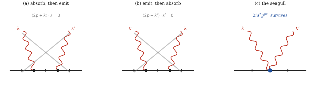
The three diagrams. (a) and (b) use the one-photon vertex twice, in the two possible orders. (c) uses the seagull once. In the target's rest frame with radiation gauge, the vertex contraction in (a) and (b) vanishes exactly, leaving only (c). That single surviving diagram is the whole of Thomson scattering.
Work in the scalar's rest frame, \(p = (m,\mathbf 0)\), choosing radiation gauge so that each polarisation has no time component, \(\varepsilon^0 = \varepsilon'^0 = 0\), while staying transverse to its own photon, \(k\cdot\varepsilon = 0\).
Now look at the vertex where the incoming photon meets the incoming scalar. The scalar leaves that vertex with momentum \(p+k\), so the rule \(-ie(p+p')^\mu\) contracts \(\varepsilon_\mu\) with \((2p+k)^\mu\):
\[ (2p+k)\cdot\varepsilon = \underbrace{2p\cdot\varepsilon}_{=\,0,\ \text{since }\varepsilon^0=0\text{ and }\mathbf p = 0} + \underbrace{k\cdot\varepsilon}_{=\,0,\ \text{transverse}} = 0 . \]Both pieces vanish separately, so this is not an approximation: the vertex is exactly zero in this frame with this gauge. The other ordering gives \((2p-k')\cdot\varepsilon'^{\,*} = 0\) the same way. Both pole diagrams are gone at tree level.
That leaves the seagull on its own. Its rule \(2ie^2g^{\mu\nu}\) contracted with the two polarisations gives
\[ \mathcal M \;\longrightarrow\; 2ie^2\,\varepsilon\cdot\varepsilon'^{\,*} = -\,2ie^2\,\boldsymbol\varepsilon\cdot\boldsymbol\varepsilon'^{\,*}, \]where the minus appears on the second form because with signature \((+,-,-,-)\) a dot product of two purely spatial vectors is minus the ordinary three-dimensional one. (Here \(\mathcal M\) means the product of the Feynman rules as written. Some books call that product \(i\mathcal M\); the difference is an overall factor that drops out when you square.)
Now turn that into a cross-section, without skipping the middle.
Square it. The sign disappears along with the \(i\), leaving \(|\mathcal M|^2 = 4e^4\,|\boldsymbol\varepsilon\cdot\boldsymbol\varepsilon'^{\,*}|^2\).
Average over the two incoming polarisations while summing over the two outgoing ones. That polarisation sum is the standard one, giving
\[ \overline{|\boldsymbol\varepsilon\cdot\boldsymbol\varepsilon'^{\,*}|^2} = \frac{1+\cos^2\theta}{2}, \]with \(\theta\) the scattering angle. Photons prefer to keep going forwards or straight back, with the sideways direction suppressed, which is why scattered sunlight is polarised.
Fold that into the usual two-body formula for a target so heavy it does not recoil. Writing \(\alpha = e^2/4\pi\), the differential cross-section is
\[ \frac{\mathrm d\sigma}{\mathrm d\Omega} = \left(\frac{\alpha}{m}\right)^2\frac{1+\cos^2\theta}{2}. \]Integrate over angles. With \(\mathrm d\Omega = 2\pi\sin\theta\,\mathrm d\theta\):
\[ \int\frac{1+\cos^2\theta}{2}\,\mathrm d\Omega = 2\pi\int_0^\pi\frac{1+\cos^2\theta}{2}\sin\theta\,\mathrm d\theta = 2\pi\cdot\frac{4}{3} = \frac{8\pi}{3}. \]So
\[ \sigma_{\rm T} = \frac{8\pi}{3}\left(\frac{\alpha}{m}\right)^2 . \]Put the electron's numbers in. The combination \(\alpha/m\) is the classical electron radius, \(2.818\) fm, so \(\sigma_{\rm T} = \tfrac{8\pi}{3}(2.818\ \mathrm{fm})^2 = 66.5\ \mathrm{fm}^2 = 0.665\) barns, which is the number quoted in every textbook for low-energy photon scattering.
Now notice what Worked example 7 really says. The answer contains the charge with the mass, nothing else. No coupling from the scalar's own interactions, no detail of what the particle is made of, no dependence on its spin. Redo it for an electron, where the diagrams are different (Dirac QED has two Compton diagrams where the scalar had three, since there is no seagull). For the same charge with the same mass you get the same \(\sigma_{\rm T}\).
That universality is a low-energy theorem, which is the EFT idea in its purest form. In the leading low-energy limit, the scattering of a photon off a slow charged particle is fixed by its charge with its mass, so any two theories agreeing on those two numbers agree on \(\sigma_{\rm T}\). The differences between them hide in the corrections.
Be careful about how far that reaches. It is a statement about the leading term. Beyond it, a target can have a magnetic moment or a polarisability, neither of which charge conservation forbids. For a composite target such as a proton the expansion also needs the photon energy to stay below whatever internal scales it has. Universality at leading order does not mean the corrections are universal too.
The QED one: light that scatters off light
One more, since you have met QED.
In classical electrodynamics two light beams pass straight through each other. Maxwell's equations are linear, so beams simply add. In QED that is not quite true: each photon can turn briefly into an electron plus a positron, which can then feel the other beam. Light scatters off light.
Now ask what this looks like to someone working far below the electron mass, someone who has never seen an electron. They cannot make one, so their theory contains photons alone. Integrating the electron out leaves an interaction between photons built from the field strength \(F_{\mu\nu}\), the famous Euler-Heisenberg Lagrangian, whose leading piece is
\[ \Delta\mathcal L_{\rm EH} = \frac{2\alpha^2}{45\,m_e^4}\Big[(\mathbf E^2-\mathbf B^2)^2 + 7(\mathbf E\cdot\mathbf B)^2\Big]. \]You do not need the loop that produces it. Look at the dimensions instead. This operator has four powers of the field strength, so it needs a coefficient of dimension \(-4\), while the only mass available is \(m_e\). That fixes how the effect scales without doing any integral. The amplitude picks up
\[ \mathcal M_{\gamma\gamma\to\gamma\gamma}\sim\alpha^2\left(\frac{E}{m_e}\right)^4, \]so the cross-section, which is the amplitude squared with the right dimensions restored, goes as \(\sigma\sim\alpha^4E^6/m_e^8\). Visible light has \(E/m_e\sim10^{-6}\), putting \((E/m_e)^4\) near \(10^{-24}\) in the amplitude alone. That is why two torch beams pass through each other. Dimensional analysis fixed every power here. It did not fix the \(2/45\) or the \(7\), which need the actual loop.
This is the same move as before, with the electron playing the part of the heavy particle, in a theory you already have the Feynman rules for.
What this post did not tell you
One thing, deliberately, because it is a separate idea.
Throughout, the couplings were treated as fixed numbers: \(g\), \(M\), \(c\), \(G_F\). Then the Fermi check above quietly needed \(\alpha\) at the \(W\) mass rather than \(\alpha\) at zero, or it missed by 7%. Couplings are not constants. They depend on the energy at which you measure them. The rules for how they change are the renormalisation group.
The two ideas fit together. Matching fixes a coefficient near the scale where the heavy particle lives. The renormalisation group then carries that value down to the scale of your experiment.
To be fair to what you have just read: tree-level matching on its own is a real prediction, correct to its stated accuracy, which is why Fermi's theory works. Running becomes necessary once you want more precision than that, or when the gap between the two scales is large enough that the logarithms of their ratio grow big. The honest way to say it is that a coupling's value depends on the scale and the convention used to define it, while the physics does not, provided you are consistent.
If you want that, it is the next thing to read:
The Renormalisation Group: A Course for People Who Know a Little QFT
Eight parts, from block spins to running couplings. Part 8 returns to effective field theory with the running included, which is the version working physicists actually use.
Exercises
Show solution
so the second term is \(\tfrac12\cdot\frac{g^2}{4}\phi^2\cdot\left(-\frac{1}{M^4}\right)\Box\,\phi^2 = -\frac{g^2}{8M^4}\phi^2\Box\phi^2\).
Dimensions: \([\phi]=1\) and \([\Box]=2\), so the operator has dimension \(6\). The Lagrangian must total 4, so its coefficient has to carry dimension \(-2\). Check that it does: \(g\) itself has dimension 1, because \(g\Phi\phi^2\) must make 4 out of three fields of dimension 1 each. So \([g^2/M^4] = 2-4 = -2\), as required.
Show solution
The muon lifetime is measured to about one part in \(10^6\), so this sits right at the edge of visibility, which is why precision extractions of \(G_F\) from muon decay do include such corrections. For anything less precise, Fermi's theory is exact for all practical purposes.
Show solution
To separate them you need the energy dependence, though here it hides better than you would expect. The first correction involves \(s+t+u\), which for four identical scalars is fixed at \(4m^2\) by momentum conservation, so it is another constant and tells you nothing. The first term that actually varies with energy or angle is the next one, going as \((s^2+t^2+u^2)/M^6\). So the deviation from a constant appears at relative order \(E^4/M^4\) rather than \(E^2/M^2\), which makes it harder to see. Measure it anyway, at several energies, to get \(M\) on its own, after which \(|g|\) follows, though not its sign.
Failing that, you reach \(E\sim M\) and make the thing directly, at which point it stops being a guess. This is what experiments at the LHC do when they quote limits on "contact interactions": those limits are bounds on \(M\) for an assumed coupling, from precisely this logic.
Where to read more
C. P. Burgess, Introduction to Effective Field Theory, arXiv:hep-th/0701053. The standard review. The toy model of a heavy scalar integrated out at tree level is done there in detail, with the loop-level version afterwards.
R. Penco, An Introduction to Effective Field Theories, arXiv:2006.16285. Lecture notes from an ICTP school, with worked examples beyond the toy model, including chiral perturbation theory and non-relativistic QED.
I. Stewart, Effective Field Theory, MIT 8.851 on OpenCourseWare. A full graduate course. Lecture 1 is watchable early, since it works through the hydrogen argument above. Be warned that the written notes cover the second half of the course, which is soft-collinear effective theory, so they assume a great deal more than this post does.
The renormalisation group course on this site, for the running couplings this post left out.