virtools: A tool for Radiometric Calibration of DAWN VIR data
The DAWN VIR Calibration Package is essential for transforming raw data collected by the Visible and Infrared Spectrometer (VIR) onboard NASA's DAWN spacecraft into scientifically meaningful and physically accurate measurements.
The VIR instrument, which observed planetary bodies like Vesta and Ceres, records radiance data in digital numbers (DN) that are affected by various instrumental and environmental artifacts. These include detector noise, dark current, stray light, bad pixels, spectral misalignments, and radiometric inconsistencies.
Without calibration, the raw data from VIR are not directly usable for scientific analysis, as they do not accurately represent the surface reflectance of the observed bodies.
The calibration package provides a suite of algorithms and correction procedures—often derived from both pre-flight laboratory characterizations and in-flight observations—that convert these raw measurements into radiometrically calibrated, artifact-corrected data products. These are suitable for applications such as mineralogical mapping, thermal modeling, surface composition studies, and planetary geophysics.
In short, the calibration package is a critical preprocessing step that ensures data fidelity, enabling reliable interpretation of planetary surfaces and supporting high-quality scientific research.
–With calibrated sight and spectral flame, We cut through the lies that corrupt the light. Stand tall, like a Hashira of knowledge— Power up… and let this cosmic battle begin!
Introduction to the Data and it's format
To use the package, we first have to know what is the data we are working with. VIR actually uses the pushbroom method to capture images of the ceres surface in different wavelengths.
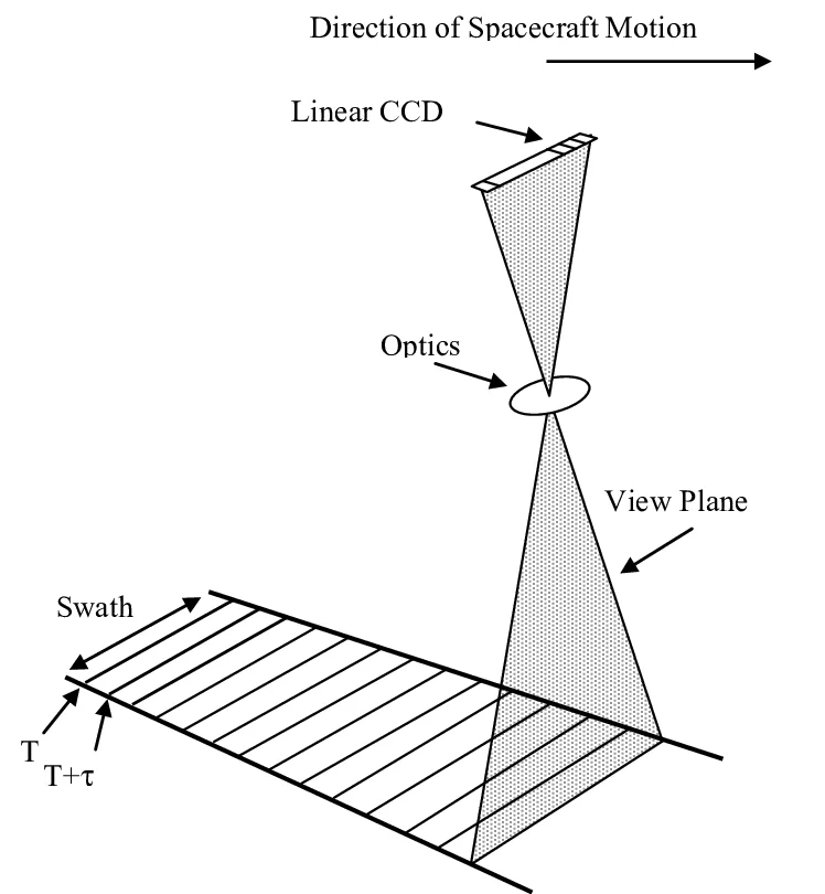
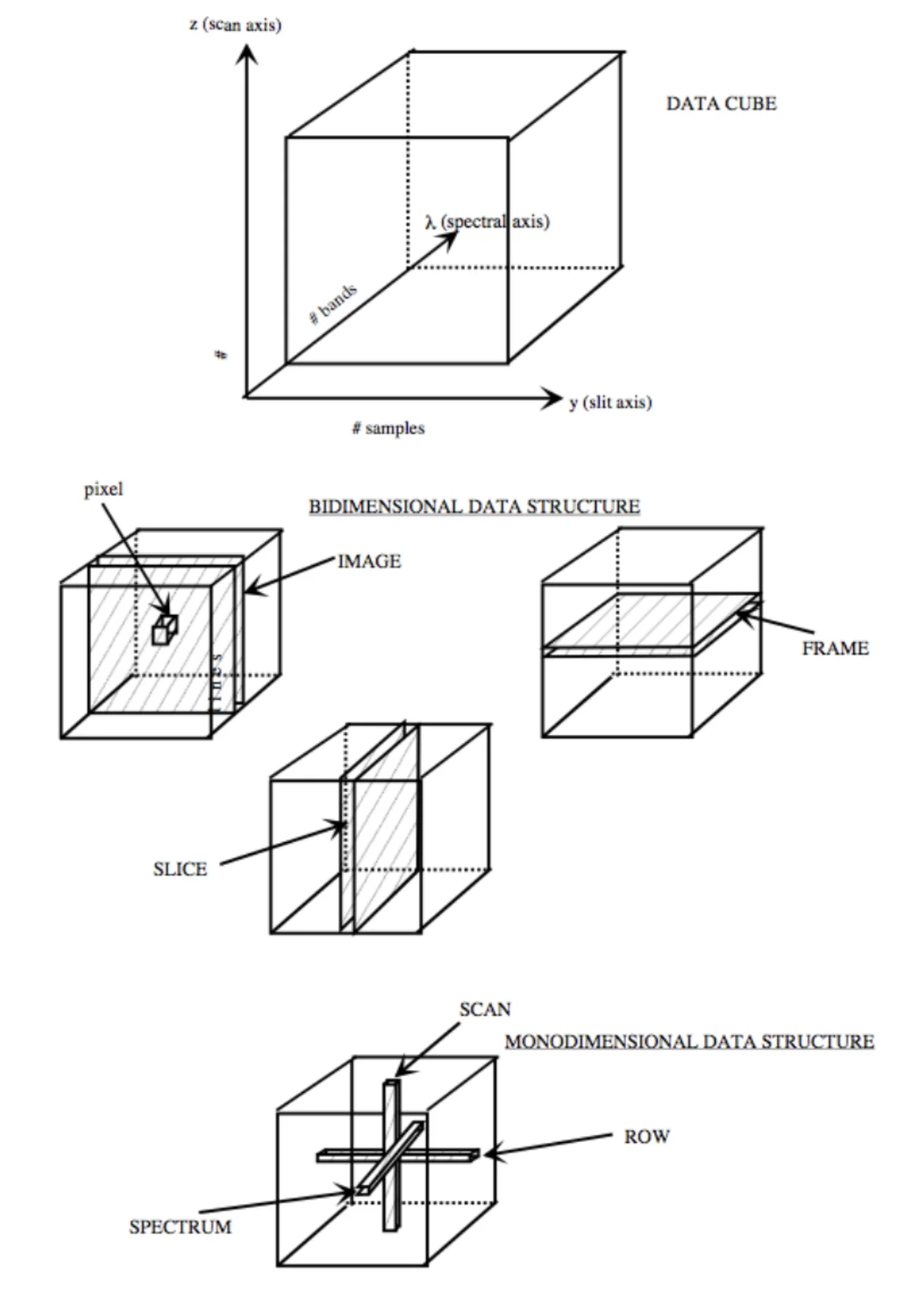
The data is stored for \(b=432\) different wavelengths, i.e., the image is taken for \(432\) different wavelengths. We can think the data as different images (sample & line) for different wavelengths stacked together. So, the image is sort of like cube as shown in the previous image. One axis is band axis, one is sample axis and other is sample axis. So, if I store the cube file data as an numpy array C, then C[b,s,l] represent the value of data for band no. \(b\), sample no. \(s\) and line no. \(l\).
| Type | Called |
|---|---|
For fixed band C[b,:,:] | Image |
For fixed sample C[:,s,:] | Slice |
For fixed line C[:,:,l] | Frame |
When the device takes the data, It generates \(4\) files:
.LBL file : This contains info about device name, target name, wavelengths, band index, SPICE file details, distance from sun and all other things. An example of the file is here.
PDS_VERSION_ID = PDS3
LABEL_REVISION_NOTE = "MTC_11-10-2011"

/* Dataset and Product Information */
DATA_SET_NAME = "DAWN VIR RAW (EDR) CERES INFRARED SPECTRA V1.0"
DATA_SET_ID = "DAWN-A-VIR-2-EDR-IR-CERES-SPECTRA-V1.0"
PRODUCT_ID = "VIR_IR_1A_1_493156585"
PRODUCT_TYPE = EDR
PRODUCER_FULL_NAME = "M. C. DE SANCTIS"
PRODUCER_INSTITUTION_NAME = "ISTITUTO NAZIONALE DI ASTROFISICA"
PRODUCT_CREATION_TIME = 2016-10-13T19:33:39.186
PRODUCT_VERSION_ID = "01"

/* File Information */
RECORD_TYPE = FIXED_LENGTH
RECORD_BYTES = 512
FILE_RECORDS = 15120
LABEL_RECORDS = 46

/* Time Information */
START_TIME = 2015-08-18T07:55:19.569
STOP_TIME = 2015-08-18T08:07:59.799
IMAGE_MID_TIME = 2015-08-18T08:01:39.684
SPACECRAFT_CLOCK_START_COUNT = "1/493156585.1098"
SPACECRAFT_CLOCK_STOP_COUNT = "1/493157346.7980"

/* Mission description parameters */
INSTRUMENT_HOST_NAME = "DAWN"
INSTRUMENT_HOST_ID = "DAWN"
MISSION_PHASE_NAME = "CERES SCIENCE HAMO (CSH)"

/* Instrument description parameters */
INSTRUMENT_NAME = "VISIBLE AND INFRARED SPECTROMETER"
INSTRUMENT_ID = "VIR"
INSTRUMENT_TYPE = "IMAGING SPECTROMETER"

/* Celestial Geometry                                       */
RIGHT_ASCENSION                  =  279.965 <degrees>
DECLINATION                      =  -62.231 <degrees>
TWIST_ANGLE                      =  227.917 <degrees>
CELESTIAL_NORTH_CLOCK_ANGLE      =  312.083 <degrees>
QUATERNION                       = (  0.11612,
                                     -0.31567,
                                     -0.91802,
                                      0.21000 )
QUATERNION_DESC                  = "
     Above parameters are calculated at the center time of the observation
     which is 2015-08-18T08:01:39.684.  The quaternion has the form:
     w, x, y, z (i.e. SPICE format)."

/* Solar geometry                                          */
SPACECRAFT_SOLAR_DISTANCE        =   441765162.5 <km>
SC_SUN_POSITION_VECTOR           = ( -259675440.2 <km>,
                                      299958230.3 <km>,
                                      194294067.4 <km> )

SC_SUN_VELOCITY_VECTOR           = ( -13.502 <km/s>,
                                      -9.829 <km/s>,
                                      -1.718 <km/s> )

/* SPICE Kernels                                            */
SPICE_FILE_NAME                  = "DAWN_CSH_R01.TM"

TARGET_NAME                      = "CAL LAMP"
TARGET_TYPE                      = "CALIBRATION"

/* COORDINATE SYSTEM                                        */
COORDINATE_SYSTEM_NAME           = "N/A"
COORDINATE_SYSTEM_CENTER_NAME    = "N/A"

/* Geometry in "IAU_VESTA" coordinates from SPICE         */
SUB_SPACECRAFT_LATITUDE          = "N/A"
SUB_SPACECRAFT_LONGITUDE         = "N/A"
SUB_SPACECRAFT_AZIMUTH           = "N/A"
SPACECRAFT_ALTITUDE              = "N/A"
TARGET_CENTER_DISTANCE           = "N/A"
SC_TARGET_POSITION_VECTOR        = ( "N/A",
                                     "N/A",
                                     "N/A" )

SC_TARGET_VELOCITY_VECTOR        = ( "N/A",
                                     "N/A",
                                     "N/A" )

LOCAL_HOUR_ANGLE                 = "N/A"
SUB_SOLAR_LATITUDE               = "N/A"
SUB_SOLAR_LONGITUDE              = "N/A"
SUB_SOLAR_AZIMUTH                = "N/A"

/* Illumination                                             */
INCIDENCE_ANGLE                  = "N/A"
EMISSION_ANGLE                   = "N/A"
PHASE_ANGLE                      = "N/A"

/* Image parameters                                         */
SLANT_DISTANCE                   = "N/A"
MINIMUM_LATITUDE                 = "N/A"
CENTER_LATITUDE                  = "N/A"
MAXIMUM_LATITUDE                 = "N/A"
WESTERNMOST_LONGITUDE            = "N/A"
CENTER_LONGITUDE                 = "N/A"
EASTERNMOST_LONGITUDE            = "N/A"
HORIZONTAL_PIXEL_SCALE           = "N/A"
VERTICAL_PIXEL_SCALE             = "N/A"
NORTH_AZIMUTH                    = "N/A"
ORBIT_NUMBER                     = "N/A"

/* Data description parameters */
PROCESSING_LEVEL_ID = "2"
DATA_QUALITY_ID = "1"
DATA_QUALITY_DESC = "0:INCOMPLETE; 1:COMPLETE"
TELEMETRY_SOURCE_ID = "EGSE"
CHANNEL_ID = "IR"
SOFTWARE_VERSION_ID = "EGSE V1.14,AMDLSpace"

/* Instrument status */
INSTRUMENT_MODE_ID = "C_H_SPE_H_SPA_F"
INSTRUMENT_MODE_DESC =
 "S_H_SPE_H_SPA_F: Science, high spectral high spatial, Full slit
  S_H_SPE_L_SPA_F: Science, high spectral low spatial, Full slit
  S_H_SPE_L_SPA_F_SUM: Science, high spectral low spatial, Summing
  S_L_SPE_H_SPA_F: Science, Low spectral high spatial, Full slit
  S_L_SPE_L_SPA_F: Science, Low spectral low spatial, Full slit
  S_L_SPE_L_SPA_F_SUM: Science, Low spectral low spatial, Summing
  S_H_SPE_H_SPA_Q: Science, high spectral high spatial, Quarter slit
  S_L_SPE_H_SPA_Q: Science, low spectral high spatial, Quarter slit
  S_H_SPE_L_SPA_F_MEA: Science, high spectral low spatial, Meaning
  S_L_SPE_L_SPA_F_MEA: Science, low spectral low spatial, Meaning
  C_H_SPE_H_SPA_F: Calibration, high spectral high spatial, Full slit
  C_H_SPE_L_SPA_F: Calibration, high spectral low spatial, Full slit
  SPARE: CALIBRATION Spare
  C_L_SPE_H_SPA_F: Calibration, low spectral high spatial, Full slit
  C_L_SPE_L_SPA_F: Calibration, low spectral low spatial, Full slit
  C_H_SPE_H_SPA_Q: Calibration, high spectral high spatial, Quarter slit
  C_L_SPE_H_SPA_Q: Calibration, low spectral high spatial, Quarter slit"
ENCODING_TYPE = "N/A"
SCAN_MODE_ID = "5"
DAWN:SCAN_PARAMETER = (0.1, 0.1, 0.26, 25)
SCAN_PARAMETER_DESC = ("SCAN_START_ANGLE", "SCAN_STOP_ANGLE",
 "SCAN_STEP_ANGLE","SCAN_STEP_NUMBER")
DAWN:SCAN_PARAMETER_UNIT = ("DEGREES", "DEGREES", "DEGREES", "DIMENSIONLESS")
FRAME_PARAMETER = (0.0, 1, 20, 0)
FRAME_PARAMETER_DESC = ("EXPOSURE_DURATION", "FRAME_SUMMING",
"EXTERNAL_REPETITION_TIME", "DARK_ACQUISITION_RATE")
DAWN:FRAME_PARAMETER_UNIT = ("S", "DIMENSIONLESS", "S", "DIMENSIONLESS")
DAWN:VIR_IR_START_X_POSITION=0
DAWN:VIR_IR_START_Y_POSITION=0
MAXIMUM_INSTRUMENT_TEMPERATURE = (84.5, 135.6, 136.6, 79.0)
INSTRUMENT_TEMPERATURE_POINT = ("FOCAL_PLANE", "TELESCOPE", "SPECTROMETER",
"CRYOCOOLER")
DAWN:INSTRUMENT_TEMPERATURE_UNIT = ("K", "K", "K", "K")
PHOTOMETRIC_CORRECTION_TYPE = "NONE"

/* Pointers to first record of objects in file */
^HISTORY = 48
OBJECT = HISTORY
END_OBJECT = HISTORY
^QUBE = "VIR_IR_1A_1_493156585_1.QUB"

/* Description of the object contained in the file */
OBJECT = QUBE

/*    Standard cube Keywords */
 AXES = 3
 AXIS_NAME = (BAND, SAMPLE, LINE)
 CORE_ITEMS = ( 432, 256, 35 )
 CORE_ITEM_BYTES = 2
 CORE_ITEM_TYPE = MSB_INTEGER
 CORE_BASE = 0.0
 CORE_MULTIPLIER = 1.0
 CORE_VALID_MINIMUM = 0
 CORE_NULL = -32768
 CORE_LOW_REPR_SATURATION = -32767
 CORE_LOW_INSTR_SATURATION = -32767
 CORE_HIGH_REPR_SATURATION = -32767
 CORE_HIGH_INSTR_SATURATION = -32767
 CORE_NAME = "RAW DATA NUMBER"
 CORE_UNIT = DIMENSIONLESS

/*  Suffix definition */
 SUFFIX_BYTES = 4
 SUFFIX_ITEMS = (    0,   0,    0)

/* Spectral axis description */

    GROUP = BAND_BIN

    BAND_BIN_CENTER =
(1.021,1.030,1.040,1.049,1.059,....)
 BAND_BIN_WIDTH  =
(0.0140,0.0140,0.0140,0.0140,......)
BAND_BIN_UNIT = MICROMETER

    BAND_BIN_ORIGINAL_BAND =
(1,2,3,4,5,6,7,8,9,10,11,12,.......)
END_GROUP = BAND_BIN

END_OBJECT                     = QUBE
END

OBJECT = HISTORY

END_OBJECT = HISTORY
.QUB file: This contains the actual data. This stores the image as Digital Number as normally happens for CCD type devices. This is the data we have to convert in radinace or reflectance. We can't directly open this data (so can't show you here).
HK_.LBL file: This contains the column names for the other data file of detail information of the device like temperature of detector, temp of spectroscope, shutter status, exposure time for each lines.
PDS_VERSION_ID                = "PDS3"
DATA_SET_ID                   = "DAWN-A-VIR-2-EDR-IR-CERES-SPECTRA-V1.0"
PRODUCT_ID                    = "VIR_IR_1A_1_493156585_HK"
PRODUCT_TYPE                  = "ENGINEERING_DATA"
PRODUCT_VERSION_ID            = "01"
PRODUCT_CREATION_TIME         = 2016-10-13T19:33:39.186

RECORD_TYPE                   = FIXED_LENGTH
RECORD_BYTES                  = 288
FILE_RECORDS                  = 35

START_TIME                    = 2015-08-18T07:55:19.569
STOP_TIME                     = 2015-08-18T08:07:59.799
SPACECRAFT_CLOCK_START_COUNT  = "1/493156585.1098"
SPACECRAFT_CLOCK_STOP_COUNT   = "1/493157346.7980"

INSTRUMENT_HOST_NAME          = "DAWN"
INSTRUMENT_HOST_ID            = "DAWN"
MISSION_PHASE_NAME            = "CERES SCIENCE HAMO (CSH)"
TARGET_NAME                   = "CAL LAMP"
INSTRUMENT_NAME               = "VISIBLE AND INFRARED SPECTROMETER"
INSTRUMENT_ID                 = "VIR"
DESCRIPTION                   = ""

^TABLE                        = "VIR_IR_1A_1_493156585_HK_1.TAB"
OBJECT                        = TABLE
  INTERCHANGE_FORMAT          = ASCII
  ROWS                        = 35
  COLUMNS                     = 33
  ROW_BYTES                   = 288
  DESCRIPTION                 = ""

  OBJECT                      = COLUMN
    NAME                      = "VERSION, TYPE, SECONDARY HEADER FLAG"
    COLUMN_NUMBER             = 1
    UNIT                      = "N/A"
    DATA_TYPE                 = ASCII_INTEGER
    START_BYTE                = 1
    BYTES                     = 2
    DESCRIPTION               = ""
  END_OBJECT                  = COLUMN

  OBJECT                      = COLUMN
    NAME                      = "APID"
    COLUMN_NUMBER             = 2
    UNIT                      = "N/A"
    DATA_TYPE                 = ASCII_INTEGER
    START_BYTE                = 4
    BYTES                     = 3
    DESCRIPTION               = ""
  END_OBJECT                  = COLUMN

  OBJECT                      = COLUMN
    NAME                      = "PACKET SEQUENCE CONTROL"
    COLUMN_NUMBER             = 3
    UNIT                      = "N/A"
    DATA_TYPE                 = ASCII_INTEGER
    START_BYTE                = 8
    BYTES                     = 5
    DESCRIPTION               = ""
  END_OBJECT                  = COLUMN

  OBJECT                      = COLUMN
    NAME                      = "PACKETS LENGTH"
    COLUMN_NUMBER             = 4
    UNIT                      = "N/A"
    DATA_TYPE                 = ASCII_INTEGER
    START_BYTE                = 14
    BYTES                     = 4
    DESCRIPTION               = ""
  END_OBJECT                  = COLUMN

  OBJECT                      = COLUMN
    NAME                      = "SCET TIME (CLOCK)"
    COLUMN_NUMBER             = 5
    UNIT                      = "N/A"
    DATA_TYPE                 = ASCII_REAL
    START_BYTE                = 19
    BYTES                     = 12
    DESCRIPTION               = ""
  END_OBJECT                  = COLUMN

  OBJECT                      = COLUMN
    NAME                      = "FRAME NUMBER"
    COLUMN_NUMBER             = 6
    UNIT                      = "N/A"
    DATA_TYPE                 = ASCII_INTEGER
    START_BYTE                = 34
    BYTES                     = 3
    DESCRIPTION               = ""
  END_OBJECT                  = COLUMN

  OBJECT                      = COLUMN
    NAME                      = "FRAME COUNT"
    COLUMN_NUMBER             = 7
    UNIT                      = "N/A"
    DATA_TYPE                 = ASCII_INTEGER
    START_BYTE                = 38
    BYTES                     = 3
    DESCRIPTION               = ""
  END_OBJECT                  = COLUMN

  OBJECT                      = COLUMN
    NAME                      = "SUBFRAME COUNT"
    COLUMN_NUMBER             = 8
    UNIT                      = "N/A"
    DATA_TYPE                 = ASCII_INTEGER
    START_BYTE                = 42
    BYTES                     = 2
    DESCRIPTION               = ""
  END_OBJECT                  = COLUMN

  OBJECT                      = COLUMN
    NAME                      = "PACKETS COUNT"
    COLUMN_NUMBER             = 9
    UNIT                      = "N/A"
    DATA_TYPE                 = ASCII_INTEGER
    START_BYTE                = 45
    BYTES                     = 2
    DESCRIPTION               = ""
  END_OBJECT                  = COLUMN

  OBJECT                      = COLUMN
    NAME                      = "SHUTTER STATUS"
    COLUMN_NUMBER             = 10
    UNIT                      = "N/A"
    DATA_TYPE                 = CHARACTER
    START_BYTE                = 48
    BYTES                     = 8
    DESCRIPTION               = ""
  END_OBJECT                  = COLUMN

  OBJECT                      = COLUMN
    NAME                      = "CHANNEL ID"
    COLUMN_NUMBER             = 11
    UNIT                      = "N/A"
    DATA_TYPE                 = CHARACTER
    START_BYTE                = 57
    BYTES                     = 3
    DESCRIPTION               = ""
  END_OBJECT                  = COLUMN

  OBJECT                      = COLUMN
    NAME                      = "COMPRESSION MODE"
    COLUMN_NUMBER             = 12
    UNIT                      = "N/A"
    DATA_TYPE                 = CHARACTER
    START_BYTE                = 61
    BYTES                     = 20
    DESCRIPTION               = ""
  END_OBJECT                  = COLUMN

  OBJECT                      = COLUMN
    NAME                      = "SPECTRAL RANGE"
    COLUMN_NUMBER             = 13
    UNIT                      = "N/A"
    DATA_TYPE                 = CHARACTER
    START_BYTE                = 82
    BYTES                     = 24
    DESCRIPTION               = ""
  END_OBJECT                  = COLUMN

  OBJECT                      = COLUMN
    NAME                      = "CURRENT MODE"
    COLUMN_NUMBER             = 14
    UNIT                      = "N/A"
    DATA_TYPE                 = CHARACTER
    START_BYTE                = 107
    BYTES                     = 12
    DESCRIPTION               = ""
  END_OBJECT                  = COLUMN

  OBJECT                      = COLUMN
    NAME                      = "CURRENT SUBMODE"
    COLUMN_NUMBER             = 15
    UNIT                      = "N/A"
    DATA_TYPE                 = CHARACTER
    START_BYTE                = 120
    BYTES                     = 14
    DESCRIPTION               = ""
  END_OBJECT                  = COLUMN

  OBJECT                      = COLUMN
    NAME                      = "IR EXPO"
    COLUMN_NUMBER             = 16
    UNIT                      = "S"
    DATA_TYPE                 = ASCII_REAL
    START_BYTE                = 135
    BYTES                     = 10
    DESCRIPTION               = ""
  END_OBJECT                  = COLUMN

  OBJECT                      = COLUMN
    NAME                      = "IR TEMP"
    COLUMN_NUMBER             = 17
    UNIT                      = "K"
    DATA_TYPE                 = ASCII_REAL
    START_BYTE                = 146
    BYTES                     = 10
    DESCRIPTION               = ""
  END_OBJECT                  = COLUMN

  OBJECT                      = COLUMN
    NAME                      = "CCD EXPO"
    COLUMN_NUMBER             = 18
    UNIT                      = "S"
    DATA_TYPE                 = ASCII_REAL
    START_BYTE                = 157
    BYTES                     = 10
    DESCRIPTION               = ""
  END_OBJECT                  = COLUMN

  OBJECT                      = COLUMN
    NAME                      = "CCD TEMP"
    COLUMN_NUMBER             = 19
    UNIT                      = "K"
    DATA_TYPE                 = ASCII_REAL
    START_BYTE                = 168
    BYTES                     = 10
    DESCRIPTION               = ""
END_OBJECT = COLUMNHK.TAB file: This contains the data corresponding to the table names in the previous HK.LBL file. It looks like,
8 102     0 1017 493156585.1020   5   1  0  1     open  IR  data_not_compressed  all_spectral_sub-frames  calibration  H_SPE_H_SPA_F   0.000000  84.482243   0.000000 170.251659   0.066178   0.997557 135.007163 137.163745  77.109671 140.777476   0.007059 142.686342  0  0  0  0  9216  1
 8 102   456 1017 493156605.1000   5   2  0  1     open  IR  data_not_compressed  all_spectral_sub-frames  calibration  H_SPE_H_SPA_F   0.000000  84.482243   0.000000 170.251659   0.066178   0.997557 135.065449 137.192888  77.672624 140.762904   0.007071 142.700913  0  0  0  0  9216  1
 8 102   912 1017 493156625.1000   5   3  0  1     open  IR  data_not_compressed  all_spectral_sub-frames  calibration  H_SPE_H_SPA_F   0.000000  84.482243   0.000000 170.222171   0.066178   0.997557 135.036306 137.178316  77.672624 140.748333   0.007383 142.686342  0  0  0  0  9216  1
 8 102  1368 1017 493156645.1000   5   4  0  1     open  IR  data_not_compressed  all_spectral_sub-frames  calibration  H_SPE_H_SPA_F   0.000000  84.513481   0.000000 170.207427   0.066178   0.997557 135.036306 137.163745  77.561390 140.748333   0.007151 142.686342  0  0  0  0  9216  1
 8 102  1824 1017 493156665.1000   5   5  0  1     open  IR  data_not_compressed  all_spectral_sub-frames  calibration  H_SPE_H_SPA_F   0.000000  84.419766   0.000000 170.236915   0.066178   0.997557 135.036306 137.178316  77.673980 140.762904   0.006509 142.686342  0  0  0  0  9216  1
 8 102  2508 1017 493156677.4550   5   1  0  1     open  IR  data_not_compressed  all_spectral_sub-frames  calibration  H_SPE_H_SPA_F   0.500000  84.513481   1.000000 170.207427   0.066178   0.997557 135.036306 137.207459  78.949101 140.704618   0.007218 142.700913  0  0  0  0  9216  2
 8 102  2964 1017 493156697.0500   5   2  0  1     open  IR  data_not_compressed  all_spectral_sub-frames  calibration  H_SPE_H_SPA_F   0.500000  84.607197   1.000000 170.222171   0.066178   0.997557 135.050877 137.178316  78.639817 140.748333   0.006668 142.671770  0  0  0  0  9216  2
 8 102  3420 1017 493156717.0500   5   3  0  1     open  IR  data_not_compressed  all_spectral_sub-frames  calibration  H_SPE_H_SPA_F   0.500000  84.544720   1.000000 170.207427   0.066178   0.997557 135.036306 137.149173  78.641173 140.762904   0.006601 142.671770  0  0  0  0  9216  2
 8 102  3876 1017 493156737.0500   5   4  0  1     open  IR  data_not_compressed  all_spectral_sub-frames  calibration  H_SPE_H_SPA_F   0.500000  84.607197   1.000000 170.207427   0.066178   0.997557 135.036306 137.222031  78.753764 140.704618   0.007065 142.715485  0  0  0  0  9216  2
 8 102  4332 1017 493156757.0500   5   5  0  1     open  IR  data_not_compressed  all_spectral_sub-frames  calibration  H_SPE_H_SPA_F   0.500000  84.669674   1.000000 170.222171   0.066178   0.997557 135.050877 137.163745  78.578774 140.748333   0.007206 142.700913  0  0  0  0  9216  2
 8 102  4788 1017 493156769.1400   5   1  0  1   closed  IR  data_not_compressed  all_spectral_sub-frames  calibration  H_SPE_H_SPA_F   0.500000  84.669674   1.000000 170.207427   0.066178   0.997557 135.021734 137.178316  79.014214 140.748333   0.007169 142.686342  0  0  0  0  9216  3
 8 102  5244 1017 493156789.0500   5   2  0  1   closed  IR  data_not_compressed  all_spectral_sub-frames  calibration  H_SPE_H_SPA_F   0.500000  84.669674   1.000000 170.207427   0.066178   0.997557 134.992591 137.178316  78.725277 140.748333   0.007261 142.686342  0  0  0  0  9216  3
 8 102  5700 1017 493156809.0500   5   3  0  1   closed  IR  data_not_compressed  all_spectral_sub-frames  calibration  H_SPE_H_SPA_F   0.500000  84.669674   1.000000 170.207427   0.066178   0.997557 135.007163 137.207459  78.726633 140.777476   0.007187 142.715485  0  0  0  0  9216  3
 8 102  6156 1017 493156829.0500   5   4  0  1   closed  IR  data_not_compressed  all_spectral_sub-frames  calibration  H_SPE_H_SPA_F   0.500000  84.607197   1.000000 170.222171   0.066178   0.997557 135.036306 137.163745  78.653382 140.762904   0.006601 142.686342  0  0  0  0  9216  3
 8 102  6612 1017 493156849.0500   5   5  0  1   closed  IR  data_not_compressed  all_spectral_sub-frames  calibration  H_SPE_H_SPA_F   0.500000  84.732151   1.000000 170.207427   0.066178   0.997557 135.021734 137.178316  78.722564 140.777476   0.006527 142.700913  0  0  0  0  9216  3
 8 102  6840 1017 493156921.0510   5   1  0  1     open  IR  data_not_compressed  all_spectral_sub-frames  calibration  H_SPE_H_SPA_F   0.500000  84.669674  20.000000 170.310635   0.066178   0.997557 135.021734 137.149173  78.622182 140.748333   0.007200 142.671770  0  0  0  0  9216  4
We have to use these files together to convert the data in the qub file into radiance and reflectance. Let's see now how.
Setting up the package:
First you have to install the package to install it. For now the package is written for IR data. This is quite general so it should work for the visible spectra too. But the detilt function is needed for that, which is not added for now.
To use this package, we have to first install it. For installing here is a bash script (if you want you can just directly download and use from git),
#!/bin/bash
ENV_DIR="./virtools-venv"
REPO_URL="https://github.com/aburousan/virtools.git"
CLONE_DIR="./virtools"

echo "Creating virtual environment in $ENV_DIR"
python3 -m venv "$ENV_DIR"
source "$ENV_DIR/bin/activate"

pip install --upgrade pip setuptools wheel build

echo "Cloning repo..."
rm -rf "$CLONE_DIR"
git clone "$REPO_URL" "$CLONE_DIR"
cd "$CLONE_DIR" || exit 1
pip install numpy scipy matplotlib scikit-image pvl PyWavelets
python3 -m build
pip install dist/*.whl

echo "virtools installed in virtualenv at $ENV_DIR"
echo "To activate: source $ENV_DIR/bin/activate"
This will create a environment in python and install the package there. For installing in conda, use:
#!/bin/bash

ENV_NAME="virtools-env"
PYTHON_VERSION="3.10"
REPO_URL="https://github.com/aburousan/virtools.git"
CLONE_DIR="./virtools"

echo "Creating conda environment: $ENV_NAME"
conda create -y -n "$ENV_NAME" python=$PYTHON_VERSION

source "$(conda info --base)/etc/profile.d/conda.sh"
conda activate "$ENV_NAME"

echo "Cloning repo..."
rm -rf "$CLONE_DIR"
git clone "$REPO_URL" "$CLONE_DIR"
cd "$CLONE_DIR" || exit 1

echo "Installing dependencies..."
conda install -y numpy scipy matplotlib scikit-image pip
pip install pvl PyWavelets build

python3 -m build
pip install dist/*.whl

echo "virtools installed in conda env: $ENV_NAME"
Once these two are ran, the package is installed in your system and you can just activate the environment to run the code.
Importing the data:
The data which is recored is stored in fortran format in MSB format. So, while importing we have to correct the endianness and aslo the array type. There are mainly two functions for importing data:
load_qub_from_lblis a function which takes lbl and qub file names with location. It will load a dictionary of all lbl file data and a numpy array with qun file data. It also returns a mask (depending on the optional argumentflag_mask) of the locations of the saturated and nan value pixels.load_qub_from_lbl_nameis a function which takes only the base folder and lbl file name. It will then load all four data files (lbl file data as previously, qub file data along with hk.lbl and hk.tab data file).
Example:
File_name_unc = "VIR_IR_1A_1_495681682"
base_folder_name = "/Data/rousan/Ceres_Data/DWNCHVIR_I1A-170324/DWNCHVIR_I1A/DATA/20150816_HAMO/20150909_CYCLE3/"
lbl_file_unc = base_folder_name+File_name_unc+"_1.LBL"
qub_file_unc = base_folder_name+File_name_unc+"_1.QUB"
lbl_hk_file_unc = base_folder_name+File_name_unc+"_HK_1.LBL"
tab_hk_file_unc = base_folder_name+File_name_unc+"_HK_1.TAB"
This are the file names with location. Now pass it to the function:
cube_array,lbl_data, flag_mask=load_qub_from_lbl(lbl_file_unc,qub_file_unc,return_flag_mask=True)The actual data is saved inside the cube_array array. lbl_data contains the meta data. Let's extract the datas from these python numpy aray and meta-data we will need.
bands, samples, lines = lbl_data["shape"]
wvlen_center = lbl_data["wave_length_cen"]
wvlen_width = lbl_data["wave_width"]
wvlen_band_val = lbl_data["wave_length_band_val"]
exposure_time = lbl_data["exposure_time"]
spacecraft_solar_dist = lbl_data["spacecraft_solar_dist"]
Now, we also need the data from house keeping files. For that there are some more functions:
hk = extract_hk_data(lbl_hk_file_unc, tab_hk_file_unc)
exposure_times = np.array(hk["data"]["exposure_time_ir"])
ir_temps = np.array(hk["data"]["ir_temp"])
spec_temps = np.array(hk["data"]["spect_temp"])
closed_index = hk["closed_indexes"]
If we want, we can directly use the other file to import the whole data. wvlen_center contains the wavelength values in \(\mu m\) & wvlen_band_val contains the band values (like eg:\(1,2,3,\cdots,\)). closed_index is contains the index of the lines for which the shutter was closed, hence giving us the dark frames.
Calibration
First thing after importing the data, we need to locate the defective pixels and then interpolate it. I am usingg the spline for that. There is a function for exactly that.
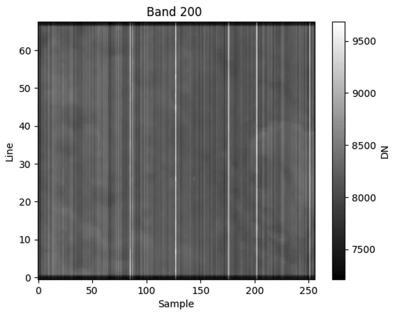
cube_def_rem = fix_defective_pixels_with_spline(cube_array,defective_ir_pixels,wvlen_center,FILTER_BANDS_IR)Here FILTER_BANDS_IR and defective_ir_pixels are numpy arraies which contains the location of filter regions(OSF regions) and detective pixel locations. This gives us an interpolated data. To see the data(image at a specific wavelength/band no.) we have a function called show_band_image.
show_band_image(cube_def_rem,200,cbar_label="DN")This gives:
After this to model thermal current, we have to use the dark frames. This will be done by using a function which will detect calibration frames in a folder.
–> –>
Hope this helps you in some way. If you like it then share with others if possible.
If you have some queries, do let me know in the comments or contact me using my using the informations that are given on the page About Me.