Finding age of the Universe using AstronomR

In the vast multiverse, where galaxies clash like titanic warriors and time itself bends to cosmic forces, one hero rises to uncover the the age of the Universe! Imagine AstronomR as kid Goku of calculations, wielding the power of R to decipher the mysteries of existence itself. It's not there yet like Super Goku but in time it will reach there

Just like Goku mastering new technique, AstronomR has just mastered the basic techniques to the fight—an arsenal of data analysis, redshift studies, and cosmic microwave background exploration. With each calculation, it channels the energy of celestial phenomena to reveal the timeline of our Universe’s grand saga.

In this blog, we’ll journey alongside AstronomR, diving into the science behind Hubble’s constant and the expansion of the cosmos. With every step, we’ll edge closer to discovering the Universe’s age!

So power up, and let’s begin this cosmic battle for knowledge!

🪶 Poem

In the silence of the starry night,
Lies the story of ancient light.
Born from a spark, so bold, so small,
Time stretched wide to cradle it all.

The CMB hums a distant tune,
Echoes of a fiery, newborn noon.
Hubble’s flow, a cosmic clue,
Guides us through the expanding view.

Oh, Universe, vast and wise,
Your age shines bright in endless skies.
With AstronomR, we seek to find,
The secret you've hidden in space and time.

📝 Note

AstronomR is a R-package developed by myself and Samrit Pramanik. To know more about it visit this blog There you will find some more functions and their application, along with the github link.

Introduction to Friedmann-Robertson-Walker(FRW) Metric

I will be assuming that readers have some basic knowledge on metric. But still to be sure, let's start by discussing a bit on it.

🧠 Defn

Metric is an object that turns coordinat distance into physical distance. It is normally represented by \(g\).

In a more rigorous sense, Metric is a tensor, which maps \(2\) vectors onto a real number. That real number tells us what is the distance between those two vectors.

Let's see this using an example:

🚧 Example

In 3-D Euclidean Space, the physical distance between two points separated by the infinitesimal coordinate distance \(dx\), \(dy\) and \(dz\) is,

\[ ds^2 = dx^2 + dy^2 + dz^2 = \sum_{i,j}^3\delta_{ij} dx^i dx^j = \sum_{i,j}g_{ij} dx^i dx^j \]

where \(x_1 = x\), \(x_2=y\) and \(x_3=z\). As, we can clearly see \(g_{ij}=\delta_{ij}\), i.e.,

\[ g_{euc} = \begin{pmatrix} 1 & 0 & 0 \\ 0 & 1 & 0 \\ 0 & 0 & 1 \end{pmatrix} \]

Let's see one more example.

🚧 Example

Let's say we have two points. They have a coordinate values \((r,\theta, \phi)\) and \((r+dr, \theta+d\theta, \phi+d\phi)\). The distance between this two points are,

\[ ds^2 = dr^2+r^2 d\theta^2+r^2 \sin^2(\theta) d\phi^2 = \sum_{i,j}^3g_{ij}dx^i dx^j \]

where \(x_1 = r\), \(x_2=\theta\) and \(x_3=\phi\). Here the metric is,

\[ g = \begin{pmatrix} 1 & 0 & 0 \\ 0 & r^2 & 0 \\ 0 & 0 & r^2 \sin^2(\theta) \end{pmatrix} \]

It should be noted that people using different coordinate systems won't necessarily agree on the coordinate distance between two points, but they will always agree on the physical distance, \(ds\), i.e., \(ds\) is an invariant.

I hope those two examples makes it clear that metric helps us to measure physical distance and in general it should depend upon the position itself, i.e., \(g=g(t,\vec{x})\).

Normally, we actally use Einstein's equation to find the metric for a given matter and energy distribution. But here we will assume a Spatial Homogeneity and Isotropy of the Universe which implies that universe can be represented by a time-ordered sequence of \(3-D\) spatial slices. The \(4-D\) line element can be written as,

\[ ds^2 = -c^2 dt^2 + a^2(t)\Big(\frac{dr^2}{1- k r^2/R_0^2}+r^2 d\Omega^2\Big) \]

where \(d\Omega^2=d\theta^2+\sin^2(\theta)d\phi^2\) and \(R_0\) is the curvature of the universe. \(k\) defines the type of the universe. If \(k=0\) it means flat universe. For \(k=1\) and \(k=-1\), we have closed and open universe respectively. The function \(a(t)\) is called scale factor, which represent the fact that our universe expands as time goes on.

📝 Note

1. AstronomR can actually do the calculation for all of those.

2. In the metric(eqn-(5)), we have a rescaling symmetry, i.e., If we simultaneously rescale \(a\), \(r\) and \(R_0\) by a constant \(\lambda\) the geometry of the spacetime remains same. We will use this freedom to set the scale factor today, at \(t=t_0\), to be unity, \(a(t_0)=1\). The scale \(R_0\) is then the physical curvature scale today.

It should be remembered throughout this blog using the subscript \(0\) to denote quantities evaluated today, at \(t=t_0\),

What Hubble Parameter and Constant?

To understand the idea of we have to remember there are two coordinates in the picture.

1. Comoving Coordinate,\(r\) (This is the coordinate of the grid. The numbers stick on the grid).

2. Physical Coordinate, \(r_{phy}=a(t)r\)(THis is the actual physical distance we measure).

In this image the lattice points are the numbers on the grid and they represent Comoving Coordinates.

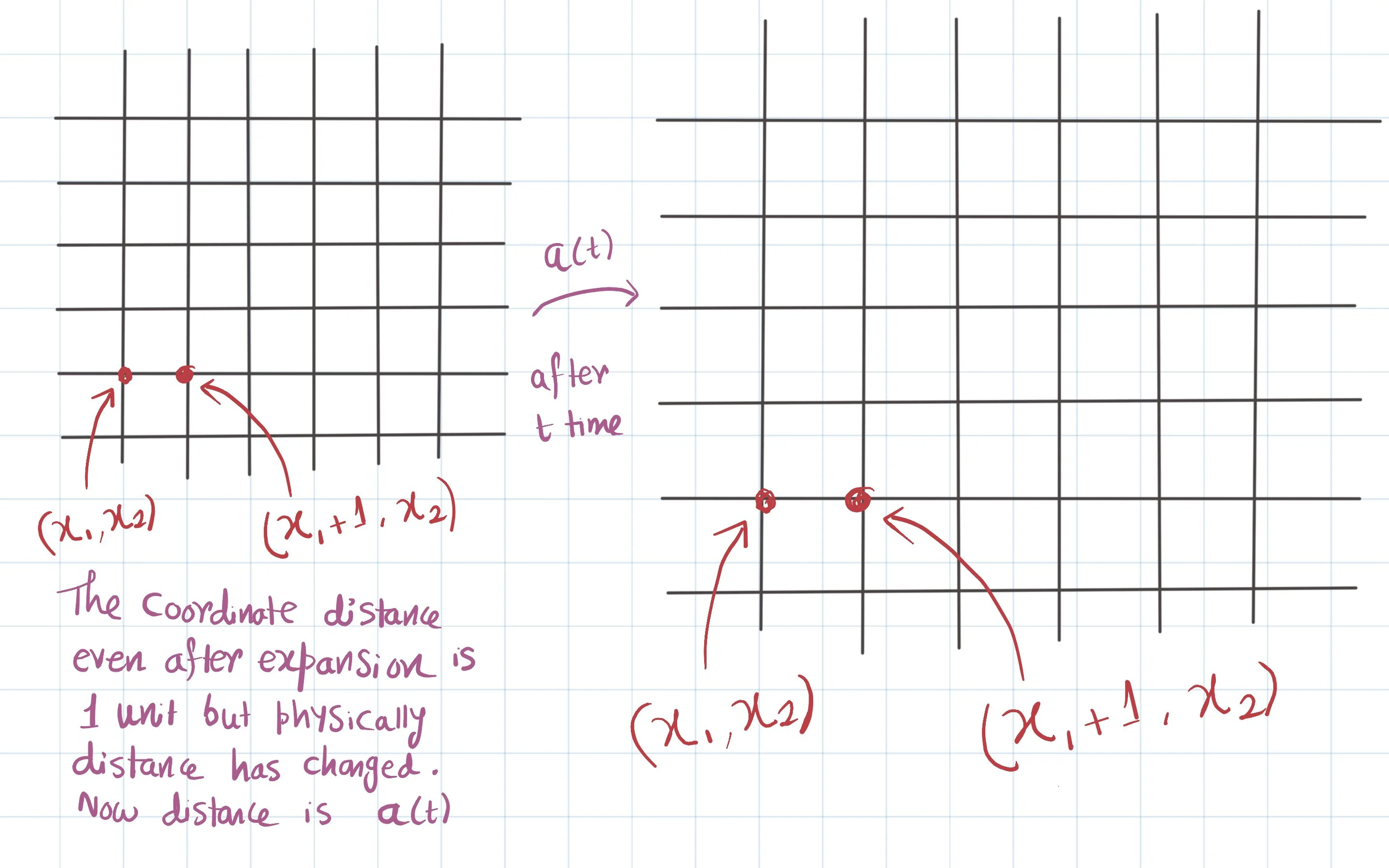
Now, let's consider a galaxy with a trajectory \(\vec{r}(t)\) in comoving coordinates and \(\vec{r}_{phy}=a(t)\vec{r}\) in physical coordinates. The physical velocity of the galaxy is,

\[ \vec{v}_{phy} = \frac{d}{dt}\vec{r}_{phy} = \frac{da}{dt}\vec{r}+a(t)\frac{d\vec{r}}{dt} = \frac{\dot{a}}{a} \vec{r}_{phy}+ \vec{v}_{pec} \]

The first term represent the velocity of the galaxy resulting from the expansion of the space between the origin and \(\vec{r}_{phy}(t)\). We can define the coefficient of \(\vec{r}_{phy}\) as Hubble Parameter, i.e.,

\[ H = \frac{\dot{a}(t)}{a(t)} \]

📝 Note

We can use something known as Redshift(\(z\)) rather than Scale Factor(\(a\)). Recall that the wavelength of light is inversely proportional to the photon energy \(\lambda = h/E\), where \(h\) is Planck's constant. We can show,

\[ \frac{1}{E}\frac{dE}{dt} = -\frac{\dot{a}}{a} \]

which implies \(E\propto a^{-1}\), the wavelength therefore scales as \(\lambda \propto a(t)\). Light emitted at a time \(t_i\) with wavelength \(\lambda_i\) will therefore be observed at a later time \(t_f\) with a larger wavelength,

\[\lambda_f = \frac{a(t_f)}{a(t_i)}\lambda_i\]

This increase of the observed wavelength is called redshift, as red light has a longer wavelength than blue. We can easily see,

\[ z+1 = \frac{a(t_0)}{a(t_i)} = \frac{1}{a(t_i)} \]

where \(a(t_0)=1\) where \(t_0\) is today's time.

At time \(t=t_0\), i.e., today, \(H(t_0) = H_0\). This is called Hubble Constant. This is written as \(H_0 = 100 h \ km\cdot s^{-1} \cdot Mpc^{-1}\), where \(h\) is a parameter with value of \(0.674\pm 0.005\). This is found from CMB anisotropy spectrum.

Setting up Friedmann Equation

Upto this point we have assumed \(a(t)\) as some unknown function of time. Now, let's invest a bit more and find some equation which tells us about \(a(t)\).

Let's start with Einstein Equation,

\[ G_{\mu \nu}=\frac{8 \pi G}{c^4}T_{\mu \nu} \]

We will take \(T_{\mu \nu}\) of the perfect fluid,

\[ T_{\mu \nu} = \Big( \rho+\frac{P}{c^2} \Big)U_\mu U_\nu + P g_{\mu \nu} \]

where \(\rho c^2\) & \(P\) are the energy density and the pressure in the rest frame of the fluid and \(U^\mu\) is its four-velocity relative to a comoving observer.

Now, using the definition of Einstein Tensor,

\[ G_{\mu \nu} = R_{\mu \nu} - \frac{R}{2}g_{\mu \nu} \]

where \(R_{\mu \nu}\) is the Ricci Tensor and \(R = R^{\mu}_{\mu}=g^{\mu \nu}R_{\mu \nu}\) is the Ricci scalar.

Now, using the formula of ricci tensor, we get,

\[\begin{aligned} R_{00} =& -\frac{3}{c^2}\frac{\ddot{a}}{a}\\ R_{ij} =& \frac{1}{c^2}\Bigg[ \frac{\ddot{a}}{a} + 2\Big( \frac{\dot{a}}{a} \Big)^2 + \frac{2 k c^2}{a^2 R_0^2} \Bigg]g_{ij}\\ R =& \frac{6}{c^2}\Bigg[ \frac{\ddot{a}}{a} + \Big( \frac{\dot{a}}{a} \Big)^2 + \frac{k c^2}{a^2 R_0^2} \Bigg] \end{aligned}\]

Using these along with \(G^{\mu}_{\nu} = g^{\mu \alpha}G_{\alpha \nu}\), we have,

\[\begin{aligned} G^0_0 =& -\frac{3}{c^2}\Bigg[ \Big( \frac{\dot{a}}{a} \Big)^2 + \frac{kc^2}{a^2 R_0^2}\Bigg]\\ G^i_j =& -\frac{1}{c^2}\Bigg[ 2\frac{\ddot{a}}{a}+ \Big( \frac{\dot{a}}{a} \Big)^2 + \frac{k c^2}{a^2 R_0^2} \Bigg]\delta^i_j \end{aligned}\]

Putting these in eqn-(11), we have,

\[ \Big(\frac{\dot{a}}{a}\Big)^2=H^2 = \frac{8\pi G}{3}\rho - \frac{k c^2}{a^2 R_0^2} \]

This is called Friedmann Equation. \(\rho\) should be understood as the sum of all contribution to the energy density of the universe. Here \(\rho = \rho_r + \rho_m + \rho_\Lambda + \rho_k\) where \(\rho_r\), \(\rho_m\), \(\rho_\Lambda\) and \(\rho_k\) corresponds to the density of radiation, matter, vacuum and curvature respectively.

In a flat universe(\(k=0\)), we have,

\[ \rho_0 = \rho_{crit,0}= \frac{3H_0^2}{8\pi G} = 1.9\times 10^{-29} h^2 gm/cm^3 \]

This is called Critical Density. Using this we can write Friedmann Equation as,

\[ \Big(\frac{H}{H_0}\Big)^2=\Omega_r a^{-4}+\Omega_m a^{-3}+\Omega_k a^{-2}+\Omega_\Lambda \]

where \(\Omega_i = \Omega_{i,0}=\rho_{i,0}/\rho_{crit,0}\) and \(i=r,m,\Lambda, \cdots\) & \(\Omega_k = -kc^2/(R_0 H_0)^2\).

Using this equation we can find the age of the universe for different cosmological model. For that, we use another form of the equation,

\[ H_0 t = \int_0^a \frac{da}{\sqrt{\Omega_r a^{-2}+\Omega_m a^{-1}+\Omega_\Lambda a^{2}+\Omega_k}} \]

Now, let's see what we get!

Determining the age of the universe using AstronomR

In AstronomR to start doing cosmological calculations, we need to first define a cosmological model using \(h,\Omega_i's\). Let's first see how:

library(astronomR)
cosmo <- astronomR:::cosmology_model(hubble_constant_fact=0.6774, curvature_crit = 0, dark_matter_crit = 0.6911, matter_crit = 0.3089, radiation_crit = 0)
print(cosmo)

$hubble_constant_fact
[1] 0.6774

$dark_matter_crit
[1] 0.69110000000000005

$matter_crit
[1] 0.30890000000000001

$radiation_crit
[1] 0

$type
[1] "FlatLCDM"

$h_per_s
[1] 2.1949477836373805e-20

As we can see as the curvature is taken to be \(0\), it is giving us a model with flat universe.

To find the age we can use the function age_of_universe which takes two parameter. The first one is some cosmological model and the second one is unit. Unit can take \(2\) values. The default is year and another one is GY or Giga-Year.

For single component universe

Let's first consider a flat matter dominated universe, i.e., only \(\Omega_m\) exist other omega's are \(0\).

In this case, we will have the model as,

cosmo <- astronomR:::cosmology_model(hubble_constant_fact=0.6774, curvature_crit = 0, dark_matter_crit = 0, matter_crit = 1, radiation_crit = 0)
print(cosmo)

$hubble_constant_fact
[1] 0.6774

$dark_matter_crit
[1] 0

$matter_crit
[1] 1

$radiation_crit
[1] 0

$type
[1] "FlatLCDM"

$h_per_s
[1] 2.194948e-20

The last value is \(h\)'s value but in seconds.

Now run,

astronomR:::age_of_universe(cosmo)

[1] 9631145240

This is the age of the universe(9.63 billion years).

📝 Note

We can actually find it analytically. It is,

\[ t_0 = \frac{2}{3H_0} \approx 9\times 10^9 \ Yr \]

This is the famous age problem. The age of a pure matter universe is shorter than that of the oldest stars. So, we can't have only matter dominated universe.

Two-Component Universe

Now, let's consider a matter and radiation dominated universe.

c1 <- astronomR:::cosmology_model(hubble_constant_fact=0.6774, curvature_crit = 0, dark_matter_crit = 0, matter_crit = 0.4, radiation_crit = 0.6)
print(c1)

$hubble_constant_fact
[1] 0.6774

$dark_matter_crit
[1] 0

$matter_crit
[1] 0.4

$radiation_crit
[1] 0.6

$type
[1] "FlatLCDM"

$h_per_s
[1] 2.194948e-20

Now, run,

astronomR:::age_of_universe(c1,unit="GY")

[1] 7.796172

The age is almost \(7.796\) GY (again the age problem). Now, let's consider matter and dark matter dominated universe.

c1 <- astronomR:::cosmology_model(hubble_constant_fact=0.6774, curvature_crit = 0, dark_matter_crit = 0.68, matter_crit = 0.32, radiation_crit = 0)
print(c1)

$hubble_constant_fact
[1] 0.6774

$dark_matter_crit
[1] 0.68

$matter_crit
[1] 0.32

$radiation_crit
[1] 0

$type
[1] "FlatLCDM"

$h_per_s
[1] 2.194948e-20

Now, run,

astronomR:::age_of_universe(c1,unit="GY")

[1] 13.67772

This gives us \(13.6\)GY or \(13.6\) billion years. I guess it's sort of correct(\(13.8\)GY actual value).

Our Universe

In our universe, we have \(\Omega_r = 8.99\times 10^{-5}\) which can be calculated using thermal properties (can also be calculated using AstronomR after the next update). Also, \(|\Omega_k|<0.01\), so we will take this as \(0\) for now(although I encourage you to put some value and see what you get).

Using this, we have,

c1 <- astronomR:::cosmology_model(hubble_constant_fact=0.6774, curvature_crit = 0, dark_matter_crit = 0.6911, matter_crit = 0.3089, radiation_crit = 8.99e-5)
print(c1)

$hubble_constant_fact
[1] 0.6774

$dark_matter_crit
[1] 0.6911

$matter_crit
[1] 0.3089

$radiation_crit
[1] 8.99e-05

$type
[1] "FlatLCDM"

$h_per_s
[1] 2.194948e-20

Now, run,

astronomR:::age_of_universe(c1,unit="GY")

[1] 13.8086

Good! As you can see the value is very close to real value.

Stay tuned for more cosmological blogs and application of our packages.

---

Hope this helps you in some way. If you like it then share with others if possible.

If you have some queries, do let me know in the comments or contact me using my using the informations that are given on the page About Me.

Go Back